Change Point Finder
Introduction on the Kinetic Change Point Algorithm
Single-molecule imaging approaches provide datasets that reveal the kinetic behavior of individual molecules within the dataset. Detailed characterisation of rate changes and pausing is possible yielding valuable information on the kinetics of processes such as transcription, translation, and motor protein precession on an immobilized target. Due to the stochastic nature of these processes the obtained trace can usually be analysed as piece-wise linear motion.
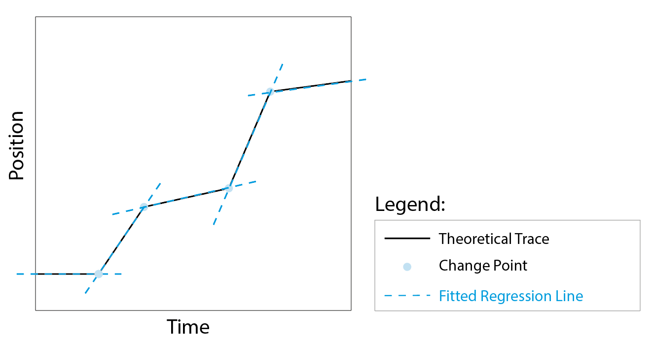
Figure 1: Theoretical trace with identified change points (blue dots) and fitted linear regression lines (blue dashed lines).
The kinetic change point (KCP) algorithm1 used in the KCP analysis tools in Mars was specifically designed to detect these different linear regions in single-molecule traces effectively. In short, the algorithm detects the change points in the trace (fig. 1, blue dots) and fits a line between the points to yield the rates for every segment (fig. 1, blue lines). The algorithm was especially developed for motion of processive single molecules having Gaussian noise and assumes piece-wise linear motion. For a detailed mathematical explanation of the model and the decision strategy the reader is referred to the paper by Hill et al.1.
Implementation of the Algorithm
The recursive binary search strategy for multiple change points (figure 2) can be visualized in three distinct steps:
- Initial sweep: Initially, the boundaries of the recorded trace are used to limit the change point search region. As soon as the first change point is identified, it is recorded and the search region is reduced accordingly. This process is repeated until the end of the trajectory is reached. This yields a first list of change points in the trajectory.
- Refinement: The positions of the identified change points are optimized locally by re-finding the change point in a smaller region around its identified location.
- Fitting: The fit parameters (start, end, slope and intercept) of the final linear segments between all change points are reported.
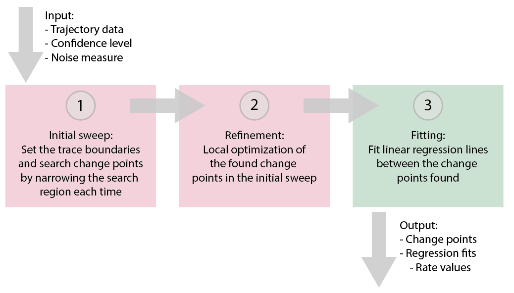
Figure 2: Visualization of the algorithm to find multiple change points.
As an introduction the reader is referred to the Kinetic Changepoint Analysis tutorial.
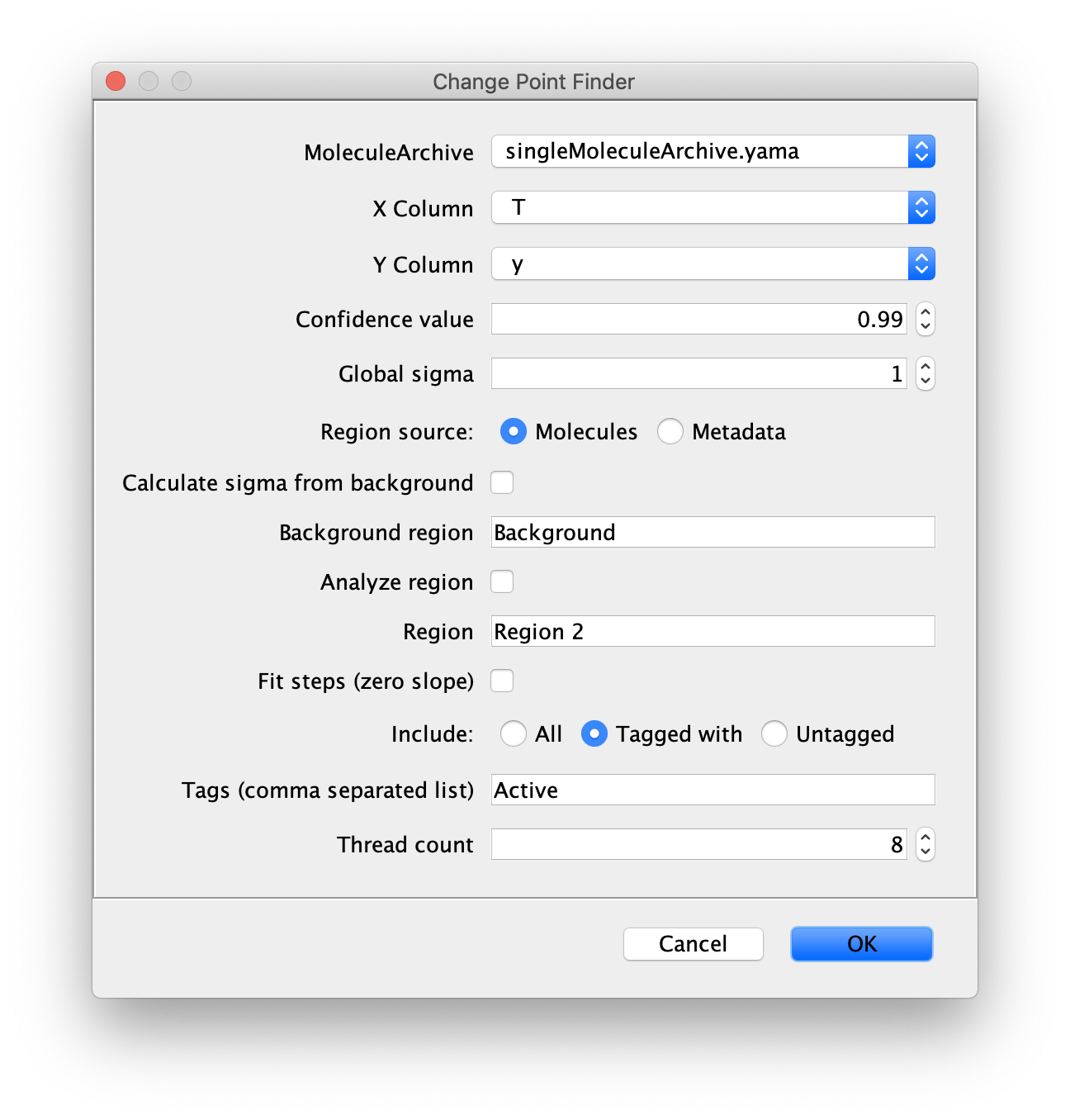
Inputs
- MoleculeArchive - Molecule Archive to find the kinetic change points for.
- X Column - X column input (f.e. time).
- Y Column - Y column input (axis along which displacement takes place).
- Confidence value - Confidence interval, used to distinguish noise from real change points.
- Global sigma - Specify the value of the error corresponding to the experimental noise to take into account.
- Region source - Set the region source to Molecules or Metadata.
- Calculate from background - Check in case the background error should be calculated from the specified background region.
- Background region - Region to calculate a background error value (sigma) from.
- Analyze region - Check box if only the region of interest has to be analyzed.
- Region - Region of the tracks to analyse. Enables the selection of a region of interest.
- Fit steps (zero slope) - Fit regression lines with a slope of 0, especially useful for fitting pauses.
- Include - Choose to include ‘all’, ‘tagged with’ or ‘untagged’ molecules in the analysis.
- Tags (comma separated list) - List of tags to base on which traces are included in the analysis.
- Thread count - Determines how much computing power of your computer will be devoted to this calculation. A higher thread count decreases computing time.
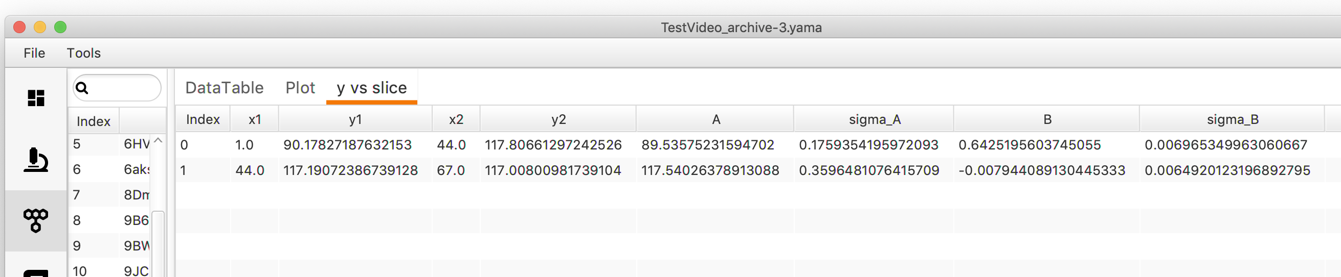
Output
- The results of KCP analysis are reported in a segments table that appears in a new sub-tab in the ‘Molecules’ tab in Rover. This table contains:
- x1: X-coordinate of segment start.
- y1: Y-coordinate of segment start.
- x2: X-coordinate of segment end.
- y2: Y-coordinate of segment end.
- A: Intercept of the line.
- sigma_A: Standard deviation from linear regression.
- B: Slope of the line (rate).
- simga_B: Standard deviation from linear regression.
How to run this Command from a groovy script
#@ MoleculeArchive archive
#@ ImageJ ij

import de.mpg.biochem.mars.molecule.*;

//Make an instance of the Command you want to run
final KCPCommand kcpCalc = new KCPCommand();

//Populates @Parameters Services etc. using the current context which we get from the ImageJ Input
kcpCalc.setContext(ij.getContext());

//Set all the input parameters
kcpCalc.setArchive(archive);
kcpCalc.setXColumn("T");
kcpCalc.setYColumn("y");
kcpCalc.setConfidenceLevel(0.99);
kcpCalc.setGlobalSigma(1.0);
kcpCalc.setRegionSource("Molecules");
kcpCalc.setCalculateBackgroundSigma(false);
kcpCalc.setAnalyzeRegion(false);
kcpCalc.setRegion(None);
kcpCalc.setFitSteps(false);
kcpCalc.setIncludeTags("Active");

//Run the Command
kcpCalc.run();
1 Hill, F.R.; Van Ooijen, A.M. & Duderstadt K.E. (2018), “Detection of kinetic change points in piece-wise linear single molecule motion”, J. Chem. Phys. 148: 123317, https://doi.org/10.1063/1.5009387