Advanced Groovy Scripting Tutorial

level: advanced, duration: 20 min

This advanced groovy scripting tutorial builds on the information discussed in the introduction to groovy scripting tutorial. For an explanation on how to run a script, script components, and some background information about main functions used during scripting the reader is referred to that tutorial.

To follow along with this tutorial open the ‘TestVideo_archive.yama’ archive in Mars that was created in the Let’s Make a Molecule Archive tutorial. Alternatively, download this archive from the mars tutorials repository.

These calculations can also be done in a Jupyter notebook with Python. This notebook is provided in the mars tutorials repository.

1. Filtering with ‘has’ functions - Calculate the dist_y_var with respect to tag category

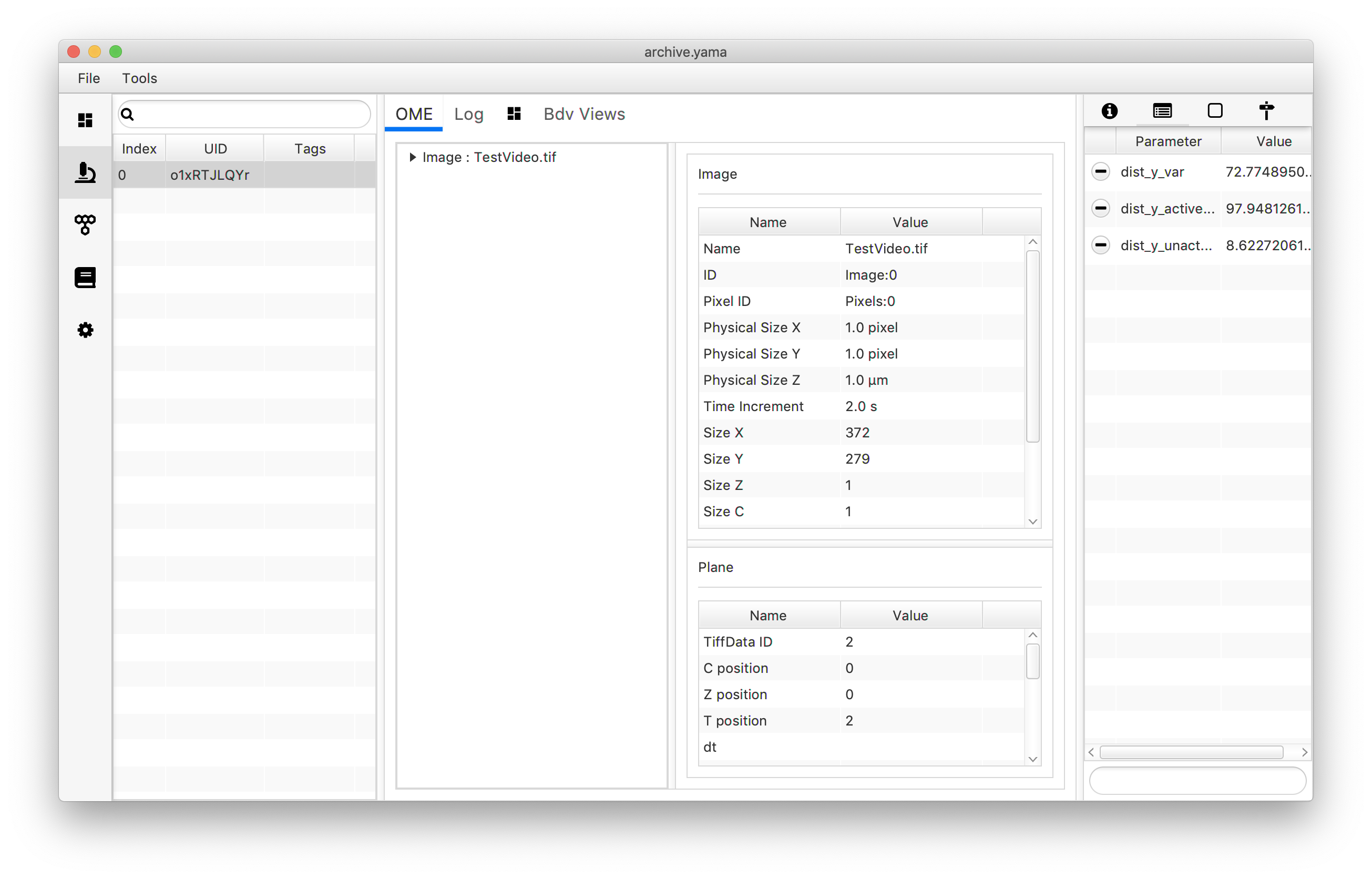
In the introduction to groovy scripting tutorial the distance travelled by each molecule in the y direction (dist_y) was calculated (section 5.1). Subsequently, the sample variance on the collection of obtained values was calculated (section 5.2). Since the data in the Molecule Archive consists of molecules showing no activity (not tagged) as well as active molecules (tagged ‘Active’) and thus large differences in the dist_y values are observed, also the calculated sample variance was very high. To get a better understanding of the variance on the dist_y parameter the variance should be calculated with respect to both categories instead yielding a variance for the tagged molecules (dist_y_active_var) as well as the untagged molecules (dist_y_unactive_var).

To do so, the script discussed in section 5.2 of the introduction to groovy scripting tutorial should be adjusted to hold a filtering step to discriminate between tagged and non-tagged molecules. For this purpose the ‘hasTag()’ function will be employed. In the script below in the first loop the ‘dist_y’ is calculated and assigned. This step can be skipped in case these values are already assigned after following the steps in the introductory tutorial.

#@ MoleculeArchive archive

import de.mpg.biochem.mars.molecule.*
import de.mpg.biochem.mars.table.*
import de.mpg.biochem.mars.util.*
import org.scijava.table.*

def list_tag = []
def list_untag = []
def list1 = []
def list2 = []

//Calculate and assign the dist_y parameter to each molecule
archive.getMoleculeUIDs().stream().forEach({UID ->
  Molecule molecule = archive.get(UID)
  MarsTable table = molecule.getTable()
  double ymin = table.min("y")
  double ymax = table.max("y")
  double dist = ymax - ymin
  molecule.setParameter("dist_y",dist)
 })

//Create a list with dist_y values for tagged and untagged molecules
archive.getMoleculeUIDs().stream().forEach({UID ->
  Molecule molecule = archive.get(UID)
  if (molecule.hasTag("Active")){
    list_tag.add(molecule.getParameter("dist_y"))
  } else {
    list_untag.add(molecule.getParameter("dist_y"))
  }
 })

//Calculate the sum, len and mean of each list
double sum_tag = list_tag.sum()
double len_tag = list_tag.size()
double mean_tag = sum_tag/len_tag

double sum_untag = list_untag.sum()
double len_untag = list_untag.size()
double mean_untag = sum_untag/len_untag

//Calculate the sample variance for both lists
for (int i = 0; i<(len_tag);i++) {
  double diff_tag = list_tag[i] - mean_tag
  double diff2_tag = diff_tag * diff_tag
  list1.add(diff2_tag)
}

for (int i = 0; i<(len_untag);i++) {
  double diff_untag = list_untag[i] - mean_untag
  double diff2_untag = diff_untag * diff_untag
  list2.add(diff2_untag)
}

double dist_tag_var = list1.sum()/(len_tag-1)
double dist_untag_var = list2.sum()/(len_untag-1)

//Assign the parameter values to the MoleculeArchive
archive.getMetadata(0).setParameter("dist_y_active_var",dist_tag_var)
archive.getMetadata(0).setParameter("dist_y_unactive_var",dist_untag_var)

The Molecule Archive generated in this tutorial can also be found in the tutorial files repository on GitHub. (TestVideo_archive_disty_advanced.yama)

The obtained values for variance are still quite high. To investigate the data and check whether a high variance has to be expected indeed, the data points of each category can be plotted in the scriptable widgets in the Rover dashboard. To do so, the bubble plot is used with a different color for the tagged and untagged categories. Visit also the tutorial and documentation on scriptable widgets.

The script for the bubble plot is based on the example in the tutorial. To visualize both populations with respect to category, the tagged population is all plotted at x=1, and the untagged population at x=2. These x-values serve purely to plot the values in distinct areas in the plot and have no data-related function whatsoever.

Note: this script is written in Groovy. Select the Groovy running language in the scripting tab of the scriptable widget before running to prevent compiling errors.

#@ MoleculeArchive archive
#@OUTPUT String xlabel
#@OUTPUT String ylabel
#@OUTPUT String title
#@OUTPUT Double xmin
#@OUTPUT Double xmax
#@OUTPUT Double ymin
#@OUTPUT Double ymax

xlabel = "Category (1=tagged, 2=untagged)"
ylabel = "Dist_y"
title = "Dist_y with respect to category"
xmin = 0.0
xmax = 3.0
ymin = -10
ymax = 35

#@OUTPUT Double[] series1_xvalues
#@OUTPUT Double[] series1_yvalues
#@OUTPUT Double[] series1_size
#@OUTPUT String[] series1_label
#@OUTPUT String[] series1_color
#@OUTPUT String series1_markerColor
#@OUTPUT Double[] series2_xvalues
#@OUTPUT Double[] series2_yvalues
#@OUTPUT Double[] series2_size
#@OUTPUT String[] series2_label
#@OUTPUT String[] series2_color
#@OUTPUT String series2_markerColor

series1_yvalues = []
series2_yvalues = []
listUID = archive.getMoleculeUIDs()

for (int i = 0; i<listUID.size();i++){
  if (archive.get(listUID[i]).hasTag("Active")){
    series1_yvalues.add(archive.get(listUID[i]).getParameter("dist_y"))
  } else {
    series2_yvalues.add(archive.get(listUID[i]).getParameter("dist_y"))
  }
}

series1_markerColor = "lightgreen"
series1_xvalues = []
series1_size = []
series1_color = []
series1_label = []
series2_markerColor = "pink"
series2_xvalues = []
series2_size = []
series2_color = []
series2_label = []

for (int i = 0; i<(series1_yvalues.size());i++) {
  series1_xvalues.add(1)
  series1_size.add(4.0)
  series1_color.add("blue")
  series1_label.add("none")
}

for (int i = 0; i<(series2_yvalues.size());i++) {
  series2_xvalues.add(2)
  series2_size.add(4.0)
  series2_color.add("red")
  series2_label.add("none")
}

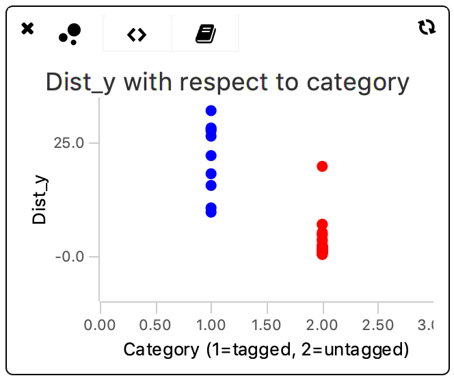
This plot shows clearly that there is quite some spread in the distance travelled in the y direction by the molecules. This difference is especially pronounced in the ‘Active’-tagged molecule category. The non-tagged category (shown in red) has one outlier with a large dist_y but apart from that data point is evenly spread around a lower dist_y value.

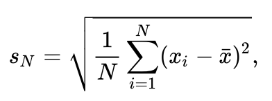
To find out if the dist_y of both categories is significantly different the standard deviation and the mean of both categories has to be calculated. To calculate the standard deviation the square root of the variance is calculated. This yields an uncorrected standard deviation as indicated in this formula. The script below adds the uncorrected standard deviation of both categories to the Molecule Archive as a new parameter.

#@ MoleculeArchive archive

//Retrieve the variance variables from the MoleculeArchive and compute the square root
double sigma_active = Math.sqrt(archive.getMetadata(0).getParameter("dist_y_active_var"))
double sigma_unactive = Math.sqrt(archive.getMetadata(0).getParameter("dist_y_unactive_var"))

//Assign the parameter values to the MoleculeArchive
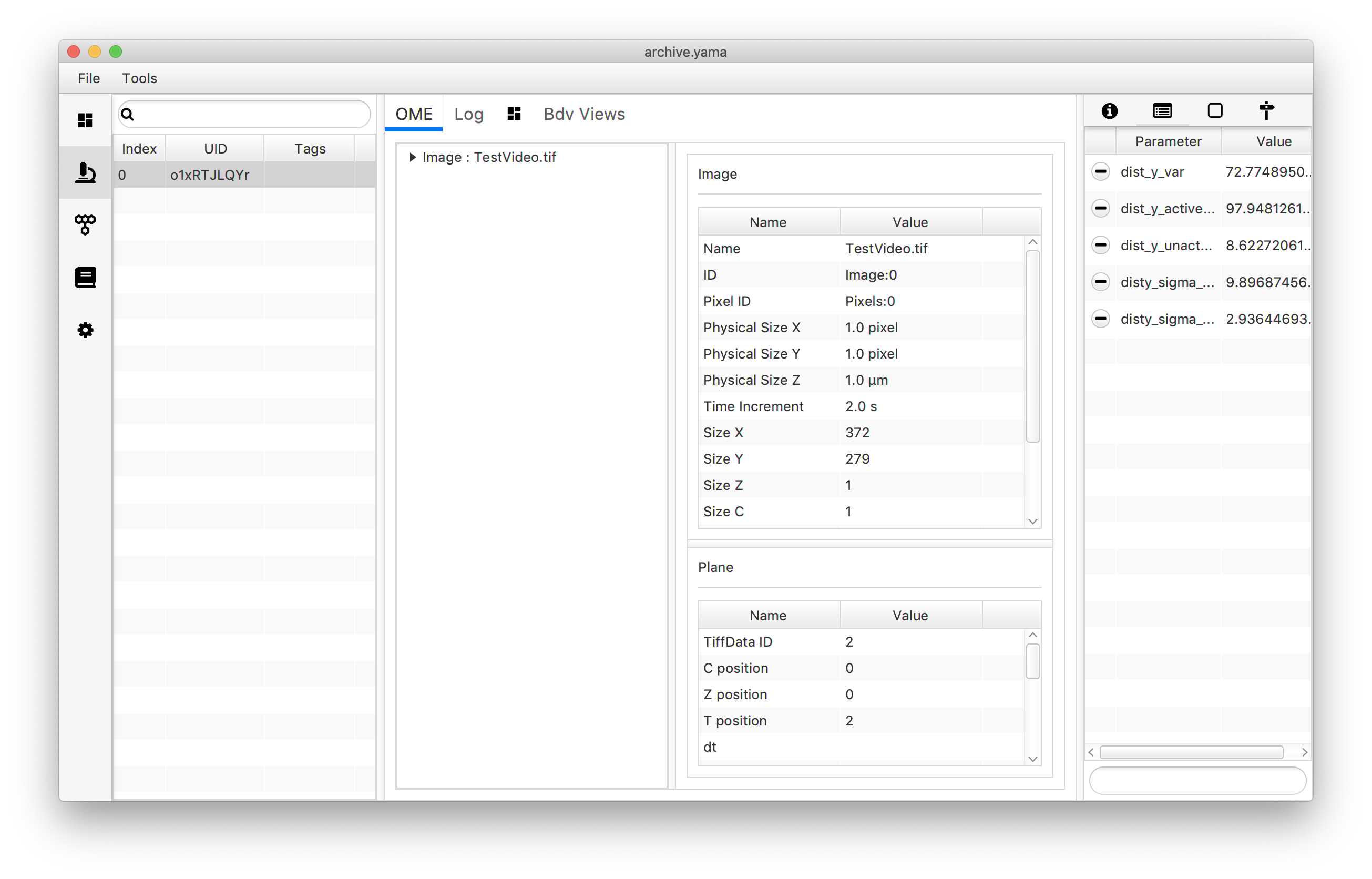
archive.getMetadata(0).setParameter("disty_sigma_active",sigma_active)
archive.getMetadata(0).setParameter("disty_sigma_unactive",sigma_unactive)

To plot the mean dist_y values and accompanying errors use the following script. In this example an XY Chart scriptable widget is used plotting the two categories as x=1 and x=2 in two different colors since this is the only chart type able to plot error bars. Note that even though this gives a good visual description of the dataset, the reader is referred to the mars to python tutorial to make better looking plots using the seaborn and MatPlotLib libraries in Python instead. Note that for this script the language option has to be set to “Groovy”.

#@ MoleculeArchive archive
#@OUTPUT String xlabel
#@OUTPUT String ylabel
#@OUTPUT String title
#@OUTPUT Double xmin
#@OUTPUT Double xmax
#@OUTPUT Double ymin
#@OUTPUT Double ymax

#@OUTPUT Double[] series1_xvalues
#@OUTPUT Double[] series1_yvalues
#@OUTPUT Double[] series1_error
#@OUTPUT Double[] series2_xvalues
#@OUTPUT Double[] series2_yvalues
#@OUTPUT Double[] series2_error
#@OUTPUT String series1_fillColor
#@OUTPUT String series1_strokeColor
#@OUTPUT Integer series1_strokeWidth
#@OUTPUT String series2_fillColor
#@OUTPUT String series2_strokeColor
#@OUTPUT Integer series2_strokeWidth

//Set global outputs
xlabel = "Category (1=Active, 2=Not Active)"
ylabel = "Dist_y"
title = "Dist_y with respect to Category"
xmin = 0.0
xmax = 3.0
ymin = -10
ymax = 35

//Set plotting settings
series1_fillColor = "blue"
series1_strokeColor = "blue"
series1_strokeWidth = 2.0
series2_fillColor = "red"
series2_strokeColor = "red"
series2_strokeWidth = 2.0

//Define the values to be plotted
series1_xvalues = [1.0]
series2_xvalues = [2.0]
series1_error = [archive.getMetadata(0).getParameter("disty_sigma_active")]
series2_error = [archive.getMetadata(0).getParameter("disty_sigma_unactive")]

listUID = []
series1_list = []
series2_list = []

archive.getMoleculeUIDs().forEach{UID -> listUID.add(UID)}

for (int i = 0; i<listUID.size();i++){
  if (archive.get(listUID[i]).hasTag("Active")){
    series1_list.add(archive.get(listUID[i]).getParameter("dist_y"))
  } else {
    series2_list.add(archive.get(listUID[i]).getParameter("dist_y"))
  }
}

series1_yvalues = [series1_list.sum()/series1_list.size()]
series2_yvalues = [series2_list.sum()/series2_list.size()]

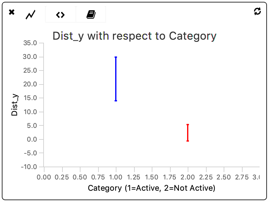
The plot shows that there is a significant (> 1x sigma) difference between the distance travelled on the y-axis by molecules within both categories. Furthermore, there is more heterogeneity within the ‘Active’-tagged category when compared to the non-tagged category.

The archive generated in this tutorial can also be found in the tutorial files repository on GitHub.

2. Groovy One Liners

A great advantage of scripting in groovy is the ability to use streams and mapping functions. In this way, longer blocks of code with loops and conditional statements (if/else) can be shortened into one liners. A few examples of such one liners are shown below.

1 Make a list of all values for one parameter defined for each molecule
This one liner loops through all molecule UIDs in the archive to find the value for the parameter called “dist_y” for all of them. These values are mapped as a double and collected in an array. This line can for example be used to plot all calculated values in the histogram widget.

#@ MoleculeArchive archive
import de.mpg.biochem.mars.molecule.*

dist_y_values = archive.getMoleculeUIDs().stream().mapToDouble{UID -> archive.get(UID).getParameter("dist_y")}.toArray()

2 Find all molecules where dist_y < 10 and tag them as “background”
In this script all values for the parameter “dist_y” are retrieved for molecules where the value of this parameter are below 10. To these molecule entries the tag “background” is added.

#@ MoleculeArchive archive

import de.mpg.biochem.mars.molecule.*
import de.mpg.biochem.mars.table.*

archive.molecules().filter{ molecule -> molecule.getParameter("dist_y") < 10}.forEach{ molecule ->
   molecule.addTag("background")
}