Let's Make A Molecule Archive - Tutorial
level: beginner, duration: 5-10 min
In this tutorial we will go through the basics of loading a video, finding and tracking peaks, navigating through Mars Rover, looking at the traces corresponding to the tracked peaks, tagging them and saving the result as a Molecule Archive (.yama) file. In the example video that is used the transcription movement of fluorescently labeled polymerase over DNA is investigated by means of TIRF microscopy. The DNA itself is not labeled and therefore is not visible in the video. This single-molecule dataset provides an excellent way to familiarise yourself with Mars and the most important plugins.
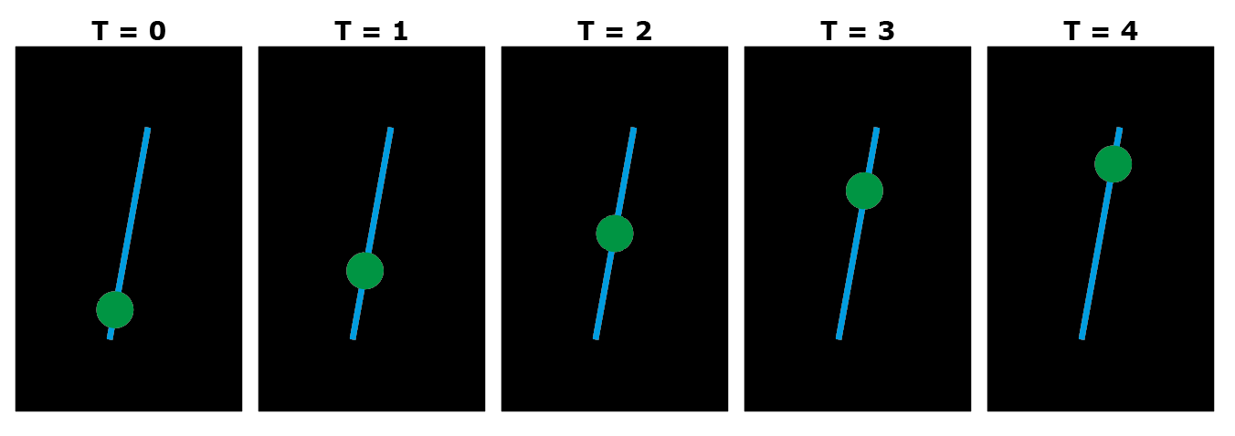
Figure 1: Schematic representation of the experiment. The DNA molecule is represented as a blue line, and the DNA polymerase as a fluorescently green dot. In the actual experiment the DNA is not fluorescently labeled and hence not visible.
1. Import a video in Fiji
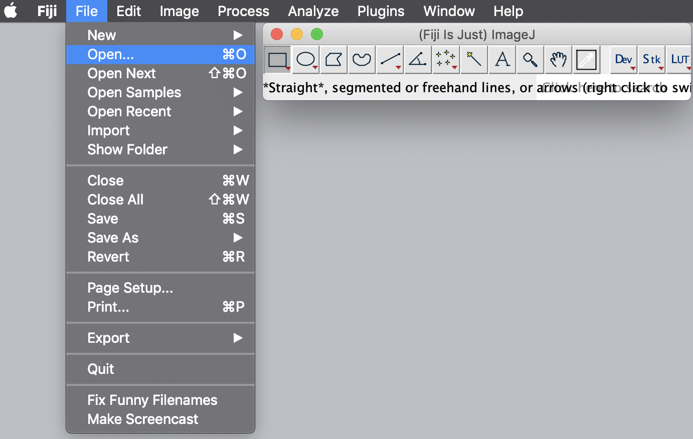
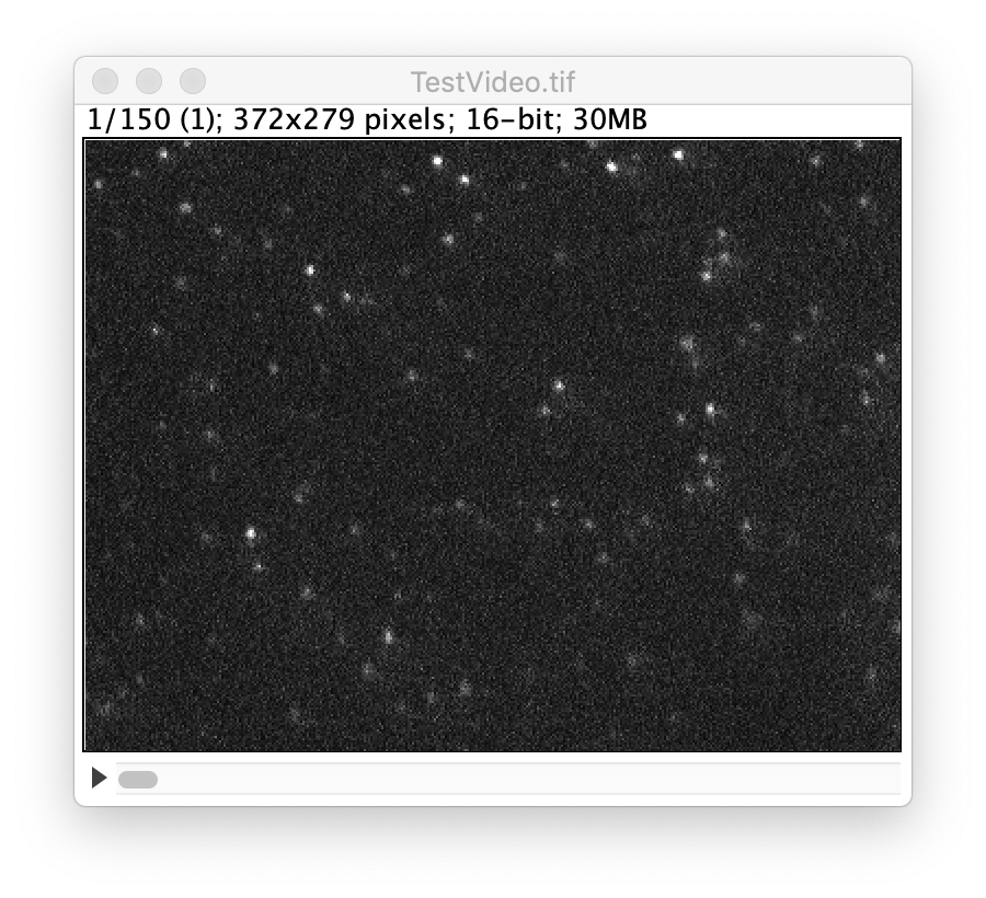
Open the example dataset ‘TestVideo.tif’ in Fiji. This will open the video in a new screen. Use the slider below the video to go through all recorded frames.
Background Information:
When playing the movie, it is clear that molecules with different behavior
are observed. The different types are listed here:
- Fast moving molecules only present in a few subsequent frames: these are molecules that are not associated with a DNA molecule and float in the buffer. Note that the buffer flow direction in this experiment is upwards whereas the transcription direction is downwards. This ensures fast flow events can be easily excluded from analysis.
- Moving molecules that travel downward slowly over a large amount of frames: these are transcribing polymerases.
- Disappearing molecules towards the end of the movie: fluorophores that are photobleached over time.
2. Use peak tracker to track peaks through frames
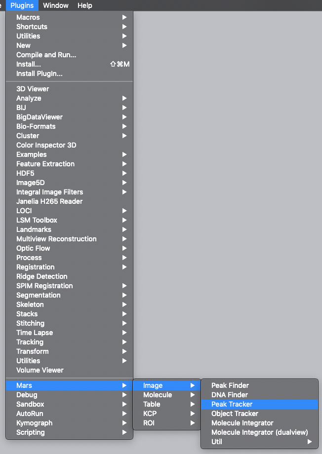
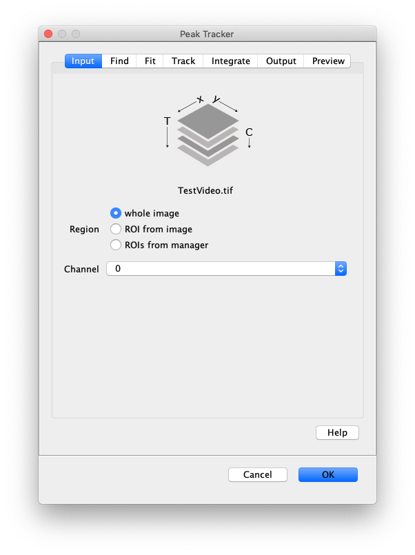
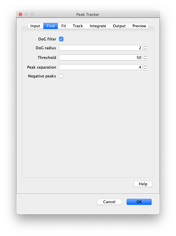
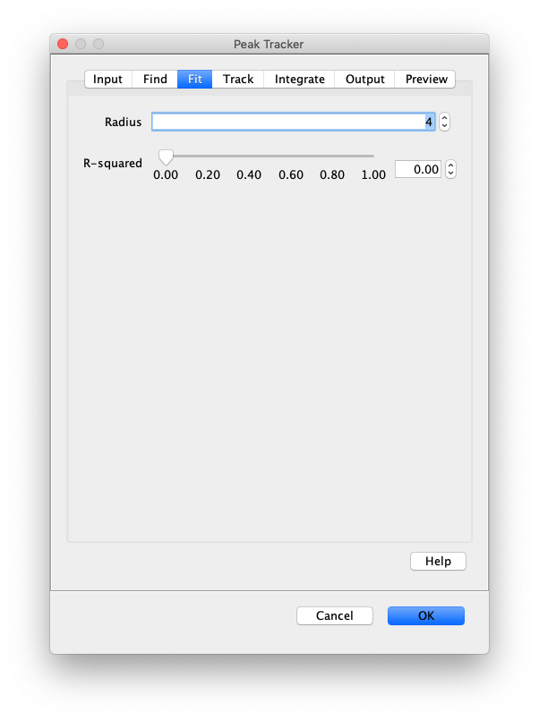
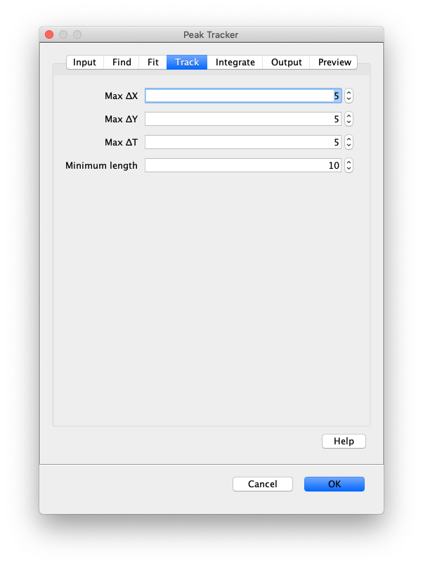
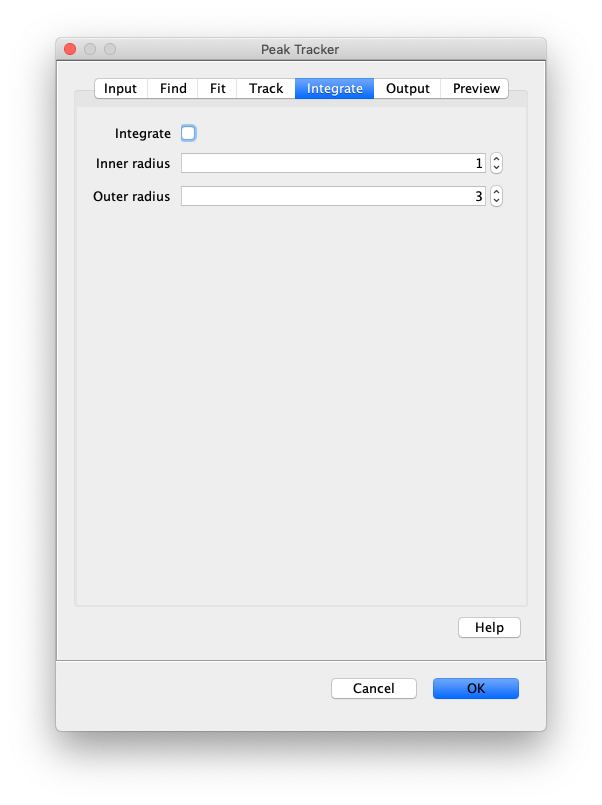
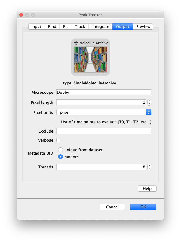
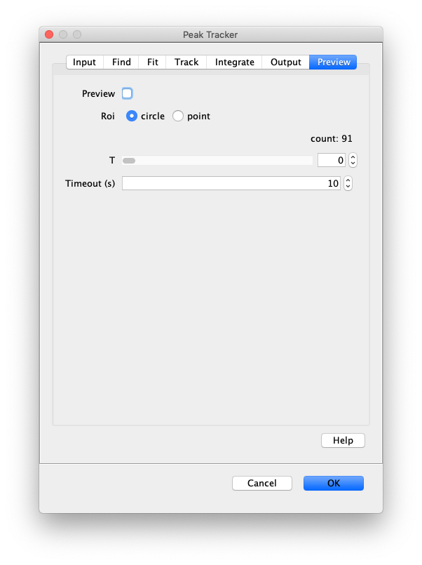
Now, open the “Peak Tracker” tool from Mars as shown and enter all settings as displayed in the screenshots below. Providing the correct settings makes sure that the tracker can find the peaks correctly. For more information about these parameters visit the documentation page.
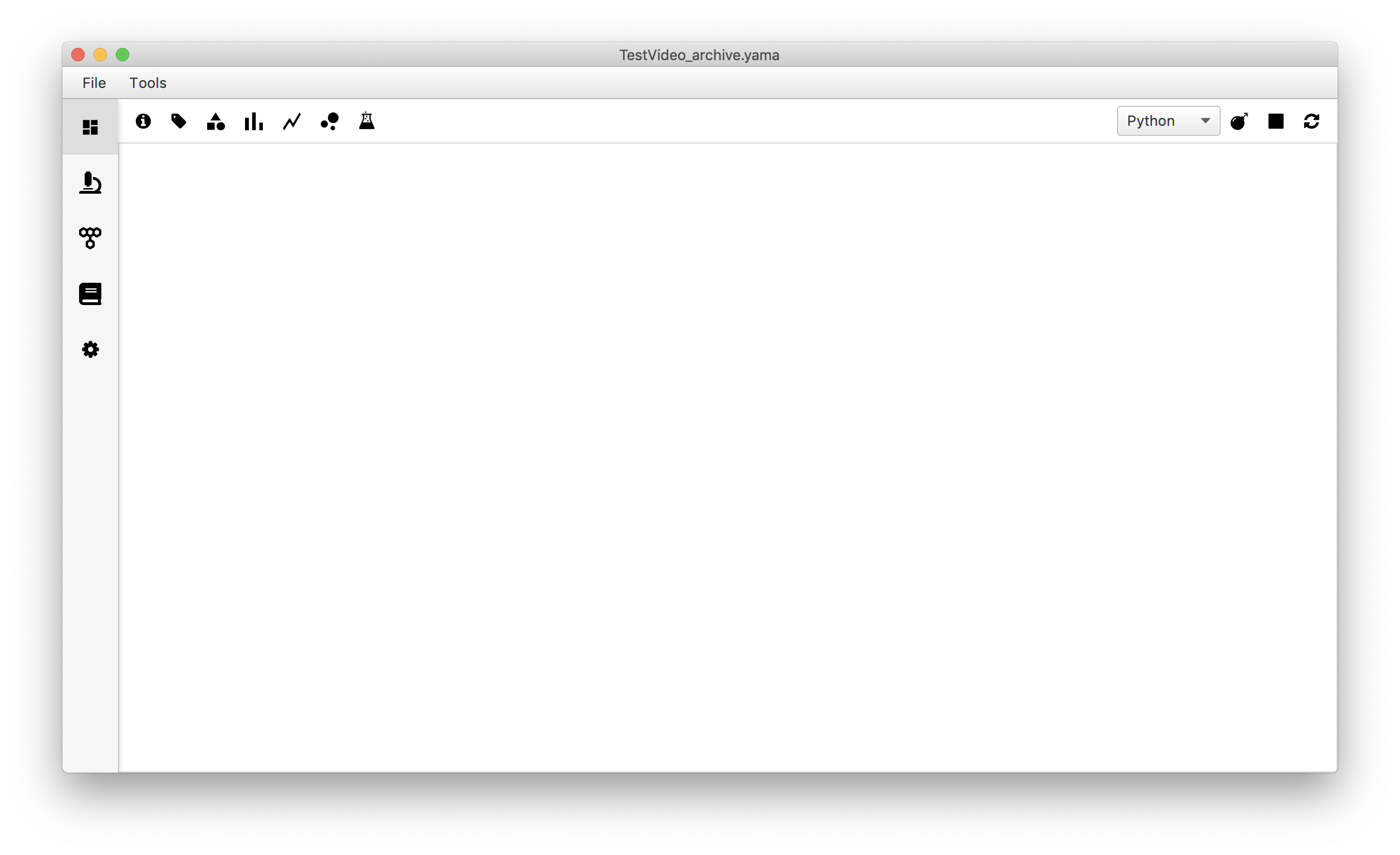
3. Navigating through Mars Rover
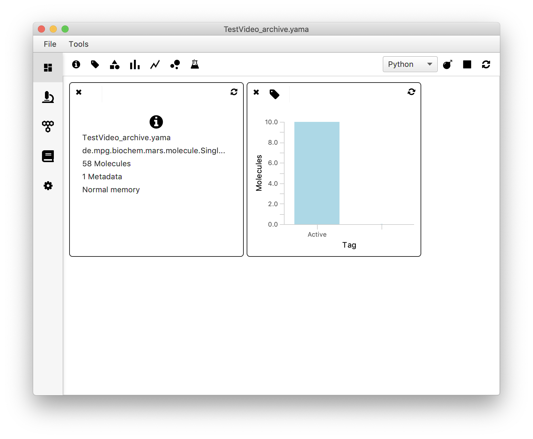
The GUI automatically opens on the desktop page. In this overview page one can see information on the dataset (press the i button), and get some statistical data. More statistical data will become available when the data is analysed in the next steps.
By using the tabs on the left, the data can be accessed. Click on the microscope icon to reveal the Metadata and Analysis log. Next to this, the ID in the left frame shows from which experiment number the data in this set originates. This number is unique for each measurement to make sure filtered data can always be traced back to the correct experiment, even when data from experiments are merged. The OME tab shows the frame numbers and the corresponding relative time when the slide was recorded. Click on each frame to display more detailed information in the middle planes.
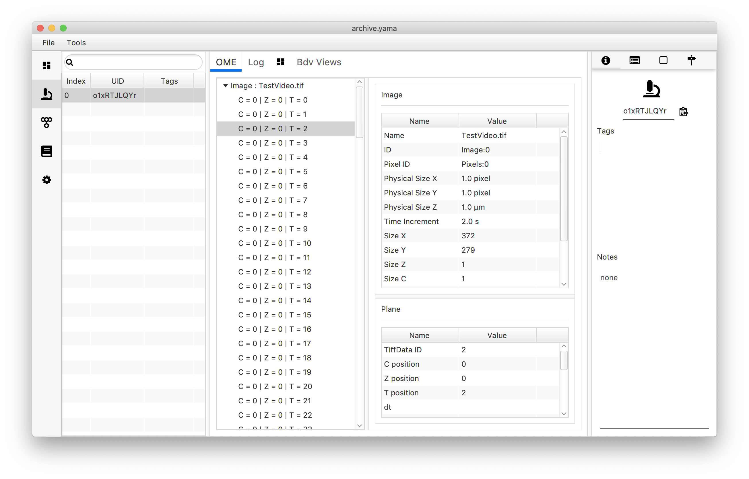
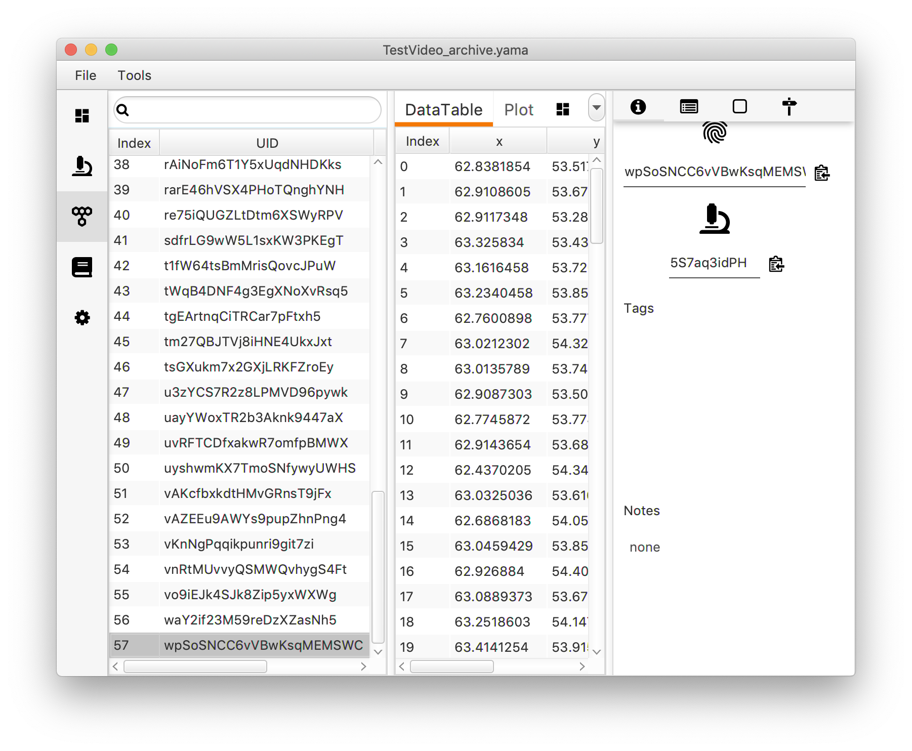
Next, open the molecule tab. This tab reveals a table with all molecules found. Each molecule is assigned an universally unique identifier (UUID) by which the molecule can be easily traced back after analysis. Click on an UUID to see the corresponding data in the adjacent “Table”. This table shows the coordinates and intensity corresponding to the tracked peak over different slides. Note that each time “Peak Tracker” is run, a new UUID will be assigned to the tracked molecule.
4. Plotting traces
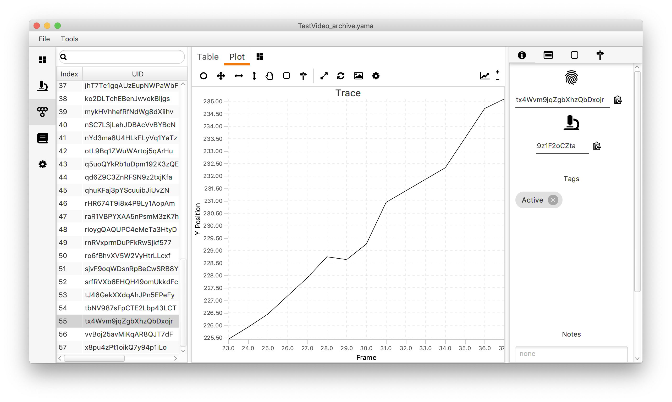
Alongside the data ‘Table’ in the molecule tab in Rover there is a tab called ‘Plot’. Switch to this tab to plot the data corresponding to the selected molecule to visualise its tracked movement.
In the top right corner, click on the plotting icon. This opens a menu that can be used to modify the plot. In this case, the settings shown make a line plot of the y position versus the frame (T). In this dataset that corresponds with the direction of transcription over the DNA plotted as a function of the time. Press the refresh button in the right corner of the menu to show the graph.
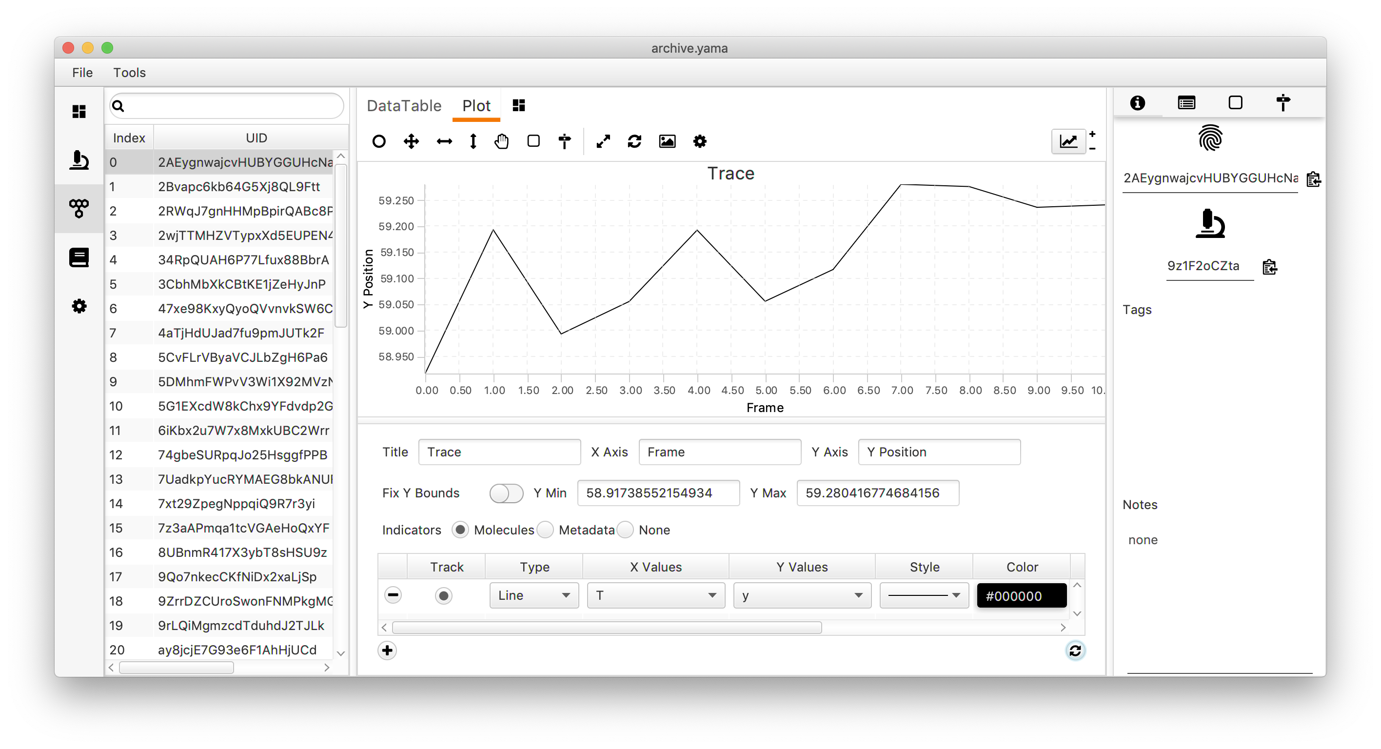
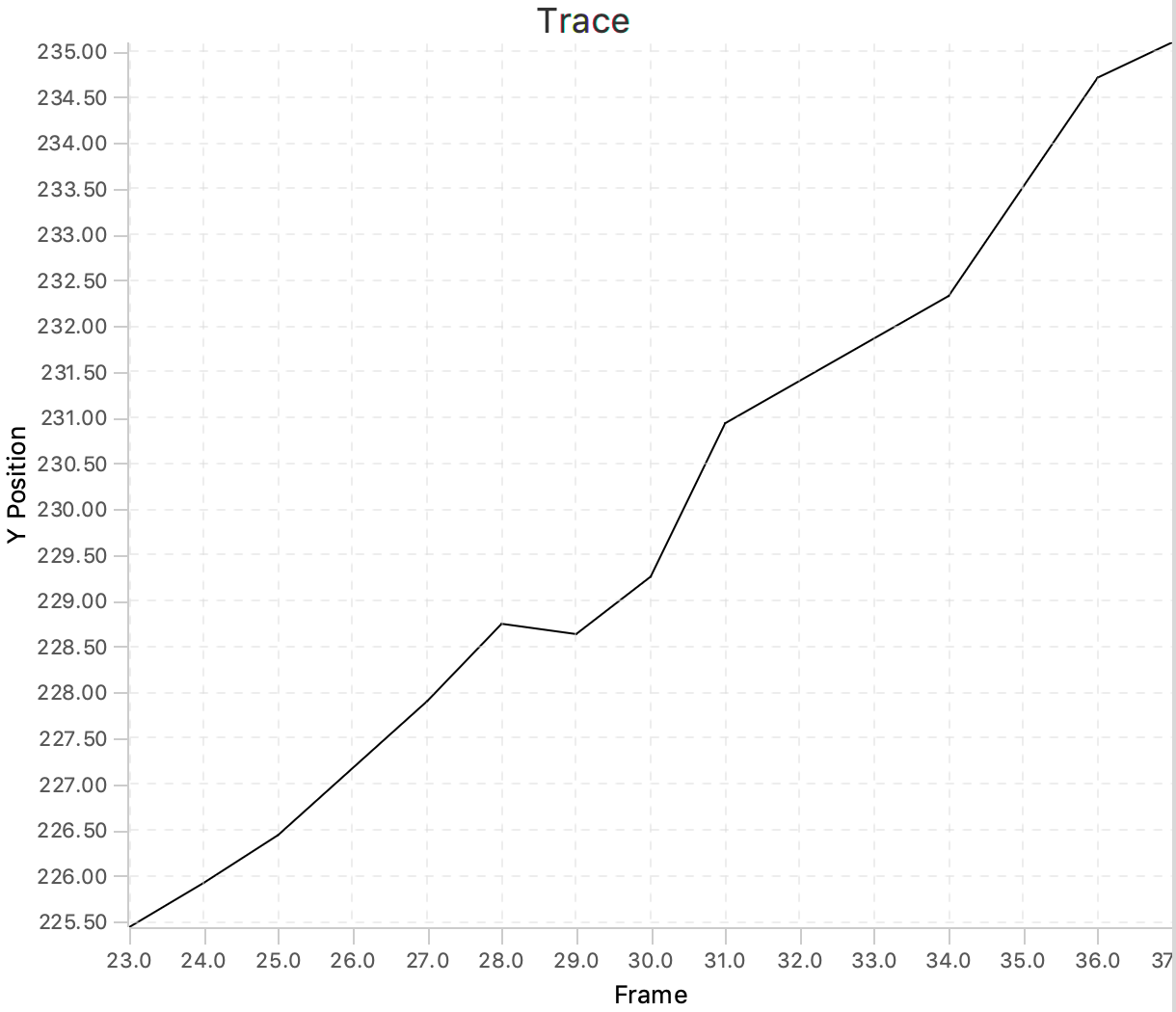
Move through the UUIDs on the left to show the plot for every molecule. As will become apparent, some molecules show a trace in which the y position almost linearly changes with the frame number. These are the molecules that are relevant for this dataset since they correspond to a polymerase that transcribes the DNA with a uniform speed. Below is an example of such a molecule. In total, this example dataset contains 10 molecules that we consider to be ‘Active’. In the next section these molecules are tagged to allow for easy filtering.
5. Tagging data
When interesting molecules in the data have been found, one can easily tag them for later reference. For now the tag name “Active” is used to filter for polymerase active molecules in further analysis. Write ‘Active’ in the Tag window on the right and press enter. If this is done correctly, a grey marked tag will show up as shown in the screenshot below. Move through all UUIDs and select all molecules fulfilling the criteria in this way.
After going through the entire dataset, go back to the desktop page of Mars Rover. Open the widget with the tag icon, refresh with the refresh button. The ‘tag plot’ now shows the amount of molecules that were tagged with a certain tag.
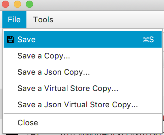
6. Saving the MoleculeArchive
The archive can be saved as a .yama file by selecting the save option. Now the data can be further analysed and plotted using Python. If you are interested in that, please continue with the tutorial on Molecule Archive data handling in Python
For more detailed information about all functions in Mars Rover please visit the documentation page.