Track the Position of a Protein on a long DNA Molecule

Many protein complexes engage and travel along DNA to perform vital functions for the cell. Single-molecule approaches can be used to study the kinetic pathways involved in these processes. This example demonstrates a complete workflow from microscopy data to kinetic information for transcription by T7 RNA polymerase at the single-molecule level.

Biological system - T7 RNA Polymerase movement on DNA
Mars workflow overview
Open the video & raw corrections
Localization & Tracking
Data correction
Merge - Build a DNA Molecule Archive
Output - Data interpretation
Conclusion
References

Biological system - T7 RNA Polymerase movement on DNA

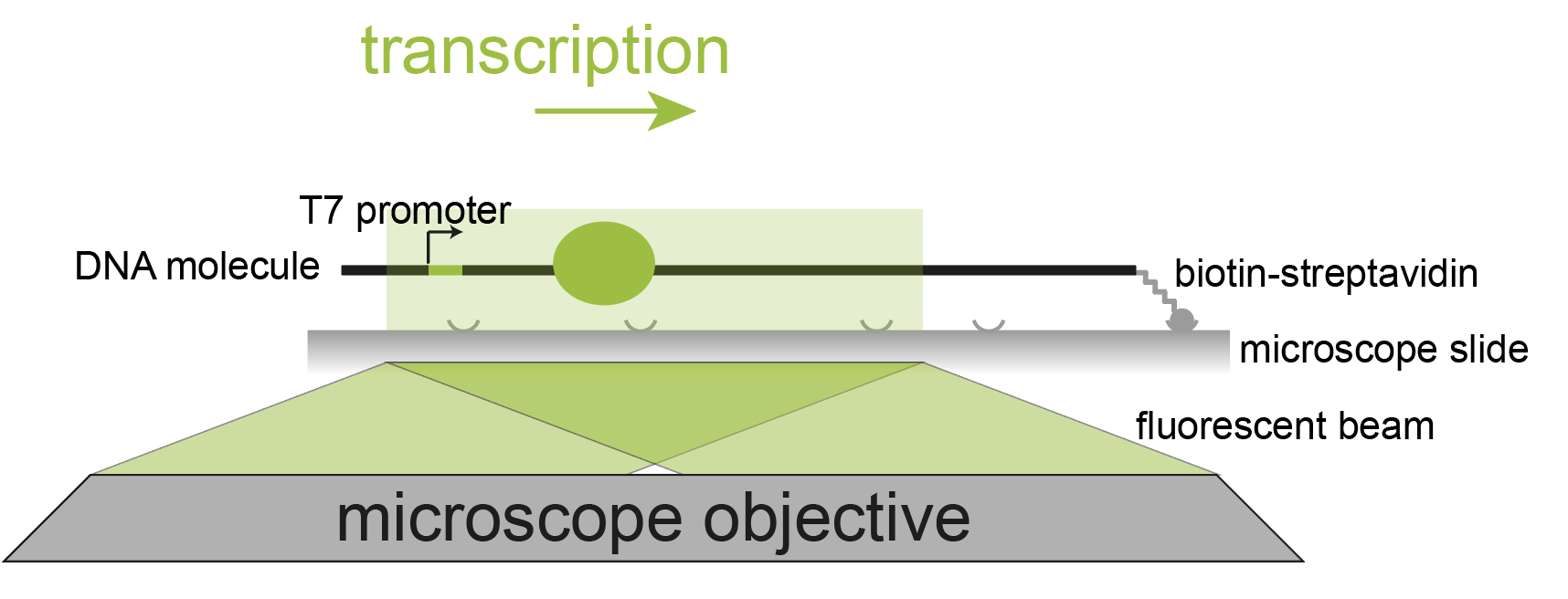
In this example, the processivity of single T7 RNA polymerase molecules on 21 kb DNA molecules is studied. The bacteriophage T7 RNA polymerase is a single-subunit DNA-dependent RNA polymerase that transcribes double-stranded DNA to RNA. Transcription is always initiated at the T7 promoter site and runs until a specific terminator is reached. ^{1, 2}

In this single-molecule experiment a fluorescently labeled T7 RNA polymerase and a 21 kb DNA template with a T7 promotor are used. The DNA template is immobilized to a functionalized glass cover slip through a streptavidin-biotin interaction. The DNA molecule is stretched by buffer flow. The RNA polymerase binds the promotor sequence on this DNA template and transcribes the template in the opposite direction of the flow. Tracking the fluorescent signal from the RNA polymerase over time enables us to follow and characterize the transcription activity of the polymerase. After transcription is completed, a fluorescent dsDNA stain is added to the buffer to visualize the individual DNA molecules in a different color. For more information on the set-up and the biological relevance please visit the paper by Scherr et al. ³

Figure 1: The set-up of the single-molecule experiment investigating movement of the T7 RNA polymerase on a 21 kb DNA molecule. Adapted from Scherr et al. ³

Mars workflow overview

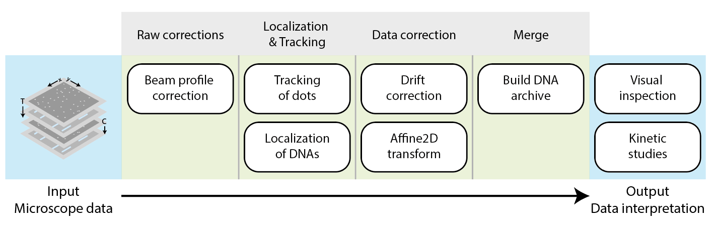
Figure 2: Flowchart showing an overview of the Mars workflow. The workflow is divided into four parts: raw corrections, localization & tracking, data correction and merge. These parts will be explained in detail below.

First, a beam correction is performed on the raw images to correct for the fluorescent signal for the gaussian beam profile. Next, the locations of the fluorescent peaks (T7 RNA polymerases) are located and tracked over time, and the DNA molecules themselves are localized. The subsequent data correction stage removes artefacts like movement through sample drift and transforms the coordinates to overlay separate DNA and polymerase channels. In the final step, the DNA and polymerase positions are merged to create a single DNA archive. This archive is then used to investigate T7 RNA polymerase movement on the DNA in the final sections of the example.

Open the video & raw image corrections

Download the video
Download the example video folder from the Github repository. The best is use git to clone the repository to your local computer. The repository uses git LFS so that should be installed as well to get the larger files. The video folder is comprised of individual TIFF files each representing one time point in an image sequence and a metadata.txt file containing the metadata information. Note that this format cannot be opened in most conventional video players. The data was collected using micromanager 1.4.

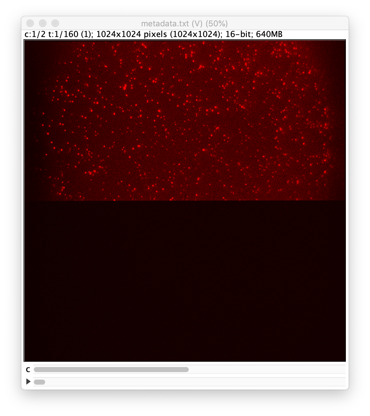
Open the video with SCIFIO
To open the video first turn the SCIFIO option on in Fiji: Edit>Options>ImageJ2, check the ‘Use SCIFIO when opening files’ option. Then open the file: use File>Open… and select the metadata file in the folder that contains the images of the video. A video viewer window opens automatically. This method ensures the Mars scifio reader for micromanager is used to open the video.

Correct for the beam profile
In most single-molecule microscopes, the excitation beam generates a gaussian profile across the image. This hinders tracking and fluorescence integration algorithms. Therefore this profile is corrected by dividing all frames by a beam profile image. To do so the Beam Profile Corrector command is used.

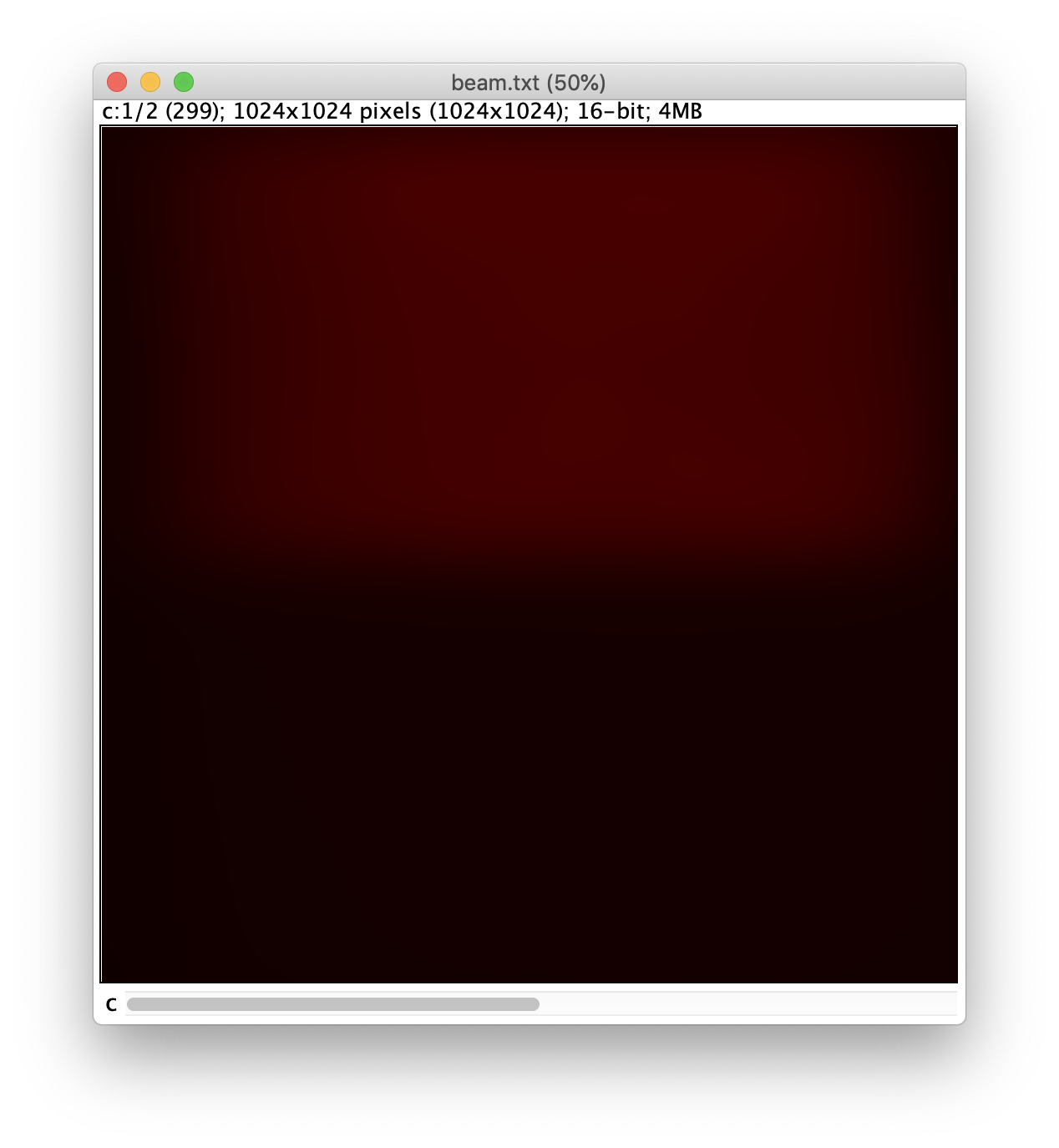
First, the beam profile image must be created. For this, the last image of channel 0 is used. To retrieve this image use Image>Duplicate… and select only frame 150. A single image should then appear that is a copy of frame 150. The image still contains many protein peaks that must be removed to build the representative image. This can be done by applying a gaussian blur with a radius of 40 (Process>Filters>Gaussian blur). The resulting image will look similar to the one shown below.

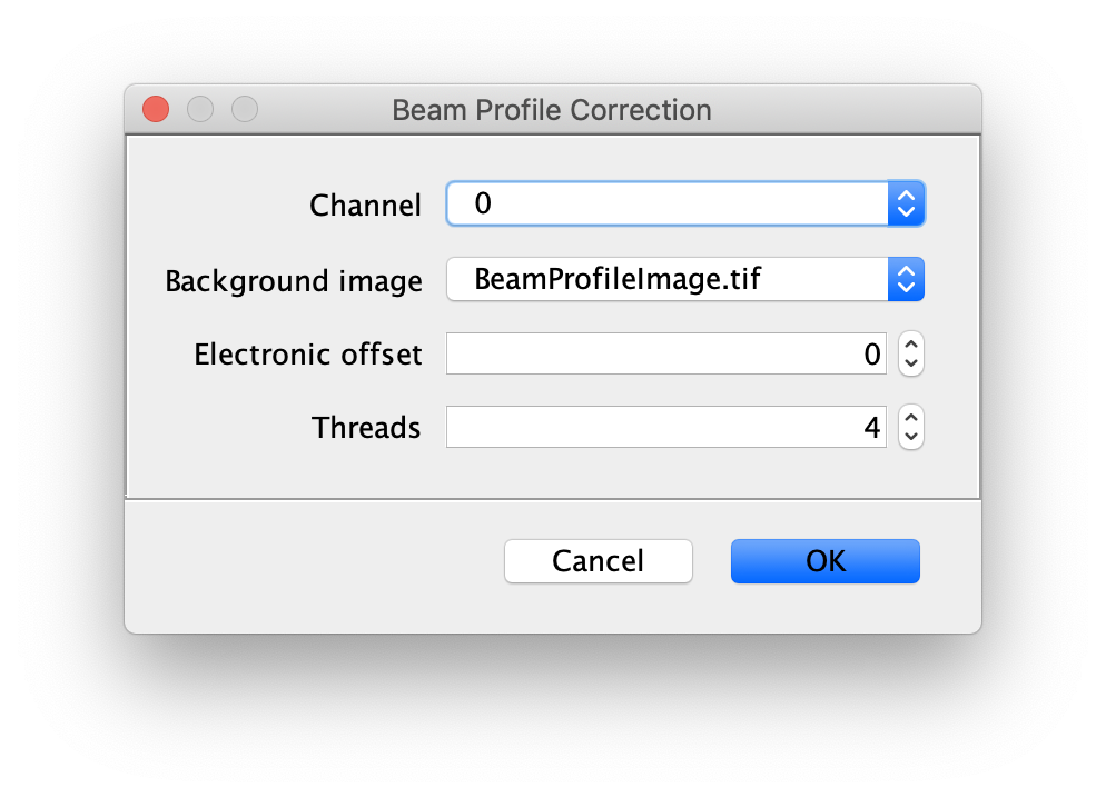
Now, run the Beam Profile Corrector command (Plugins>Mars>Image>Util). Make sure the full example video and the beam profile image are open in Fiji. Set the Channel to 0 and the background image to the profile image you have just created. The electronic offset represents the intrinsic background noise from the camera used. You can leave this set to 0 for the purposes of this example. Run the command and you will see that the protein channel has been corrected for the beam profile. Run a second time if you do not see the change due to this issue. Note that sometimes this difference is difficult to spot by eye. Beam profile correction is not essential for this example, but will make it easier to track all peaks and compare intensity values.

Localization & Tracking

Track the protein peaks to create a Single Molecule Archive
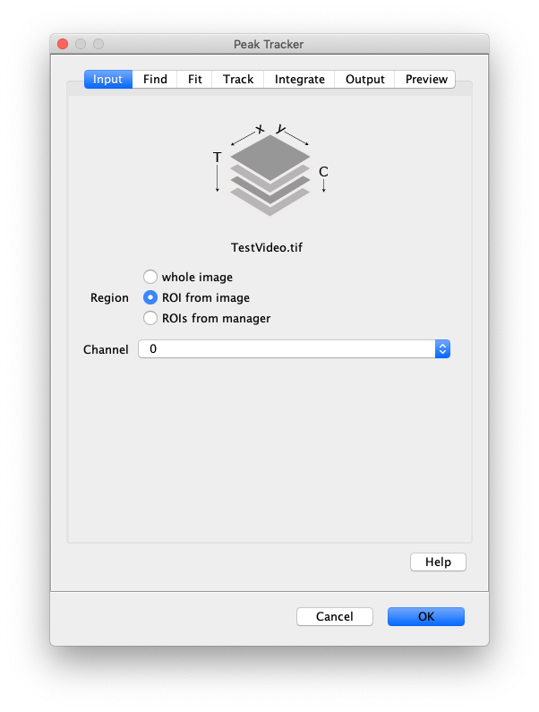
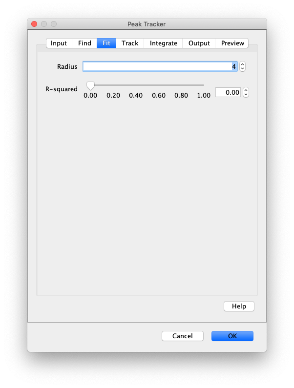
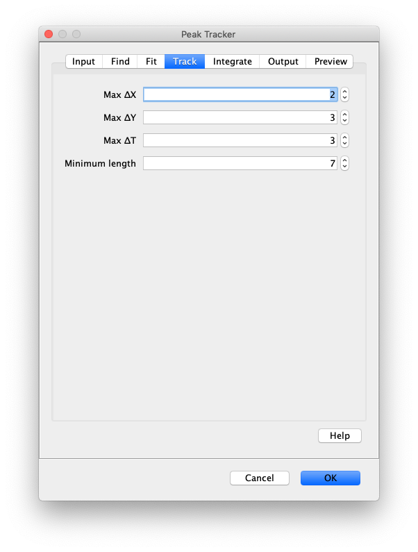
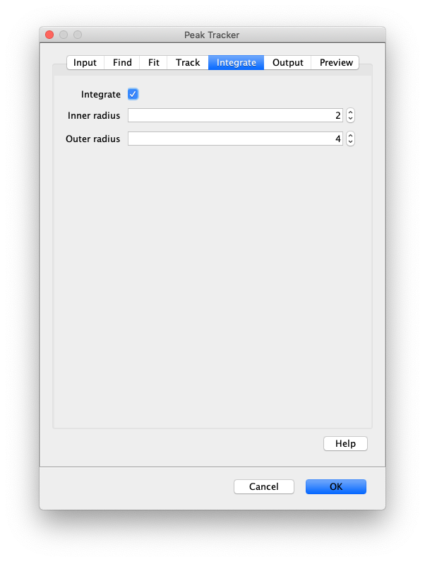
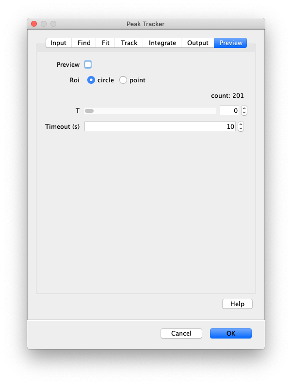
Now that the raw images has been corrected, the location of the proteins is tracked using the Peak Tracker (Plugins>Mars>Image>PeakTracker). This generates a Single Molecule Archive containing the X,Y-coordinates of each spot with respect to time. First use the ‘Rectangle’ tool in Fiji to select the region that should be processed. This should be the top half of the image that contains all the labeled polymerases. Once your selection is complete, run the Peak Tracker with the following settings:

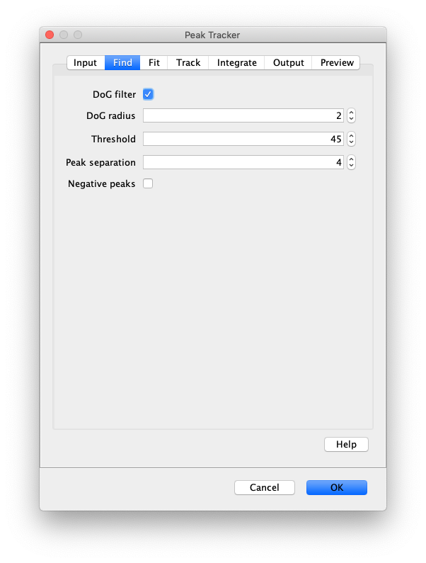
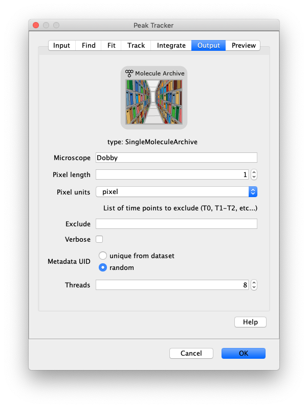
The threshold should be adjusted to ensure detection of all peaks over background. When the command is finished, a Single Molecule Archive should appear that contains all tracked molecules. Saved it with the name ‘singleMoleculeArchive.yama’.

Find and fit the DNA molecules
Now the proteins have been tracked, we can use the DNA finder (Plugins>Mars>Image>DNA Finder) to locate all DNA molecules in channel 1. This can be accomplished using the following settings:

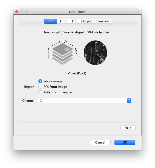
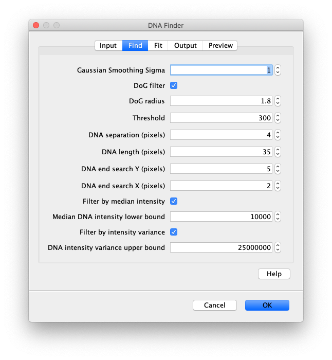
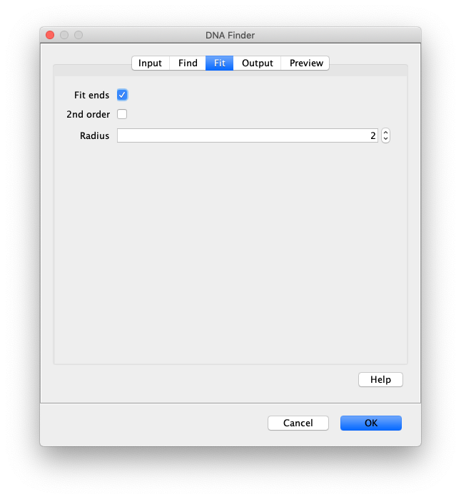
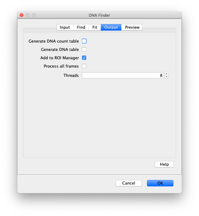
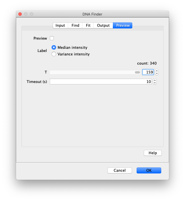
The only output should be a list of line ROIs added to the ROI Manager, each with a UID. It is very important that the time point is set to 159 since the DNA can only be seen in the last time points.

Data correction

Drift correction of the X and Y coordinates
Now that the coordinates of the polymerases and DNA molecules have been identified, a correction for sample drift in the X and Y direction can be made. Such sample drift can arise for example by slight microscope stage movement over time and would create artefacts in data analysis if not corrected.

To assess the amount of drift that occurred throughout the measurement fixed spots/stuck proteins on the surface are used. These molecules should remain at their fixed position throughout the measurement, so any deviation thereof needs to be corrected. To select for these molecules, the variance of movement is calculated for each peak. All peaks with a high variance are mobile, all peaks with a very low variance are most likely stuck on the surface and can then be tagged ‘background’. These ‘background’ molecules will then be used for drift correction.

First, calculate the variance in Y for each dot using the variance calculator (Plugins>Mars>Molecule>Util). Name the parameter ‘Y_var’. After running the command, run the short script below to automatically tag all molecules with a low Y_var as ‘background’. Use the script editor to run the script and select ‘Groovy’ as the running language.

#@ MoleculeArchive archive

archive.molecules().filter{ m -> m.getParameter("Y_var") < 1}.forEach{ m -> m.addTag("background") }

Now run the drift corrector command and supply the settings as shown below. We use the ‘singleMoleculeArchive.yama’ as an input to drift correct the tracks of the polymerases.

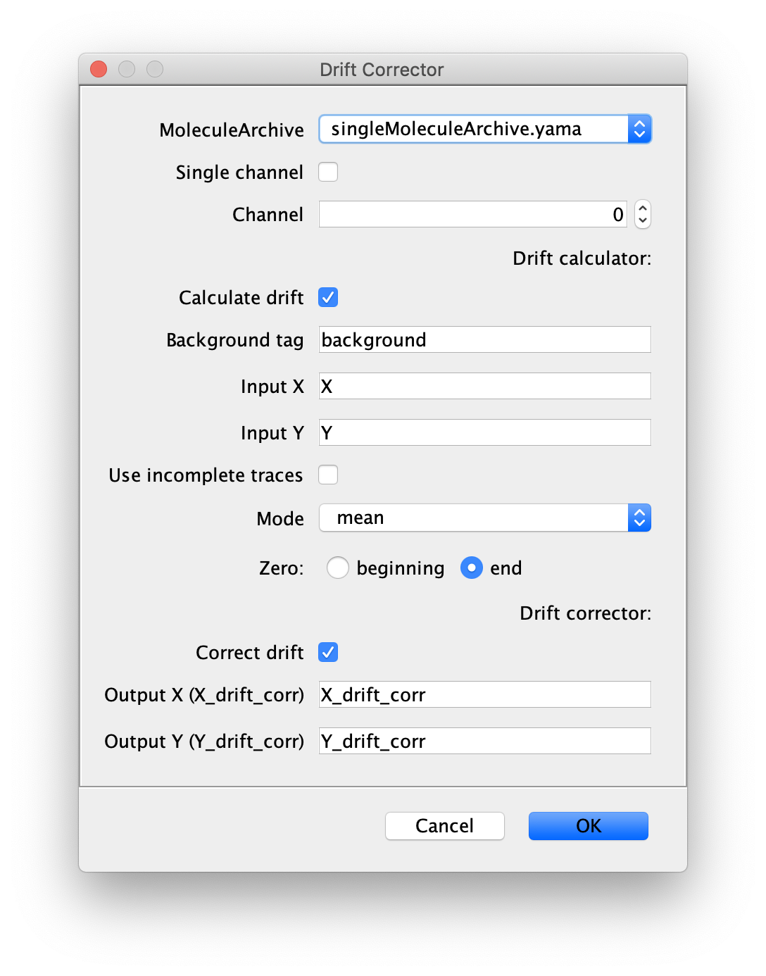
Output columns should be X_drift_corr and Y_drift_corr. The origin or zero should be the last time point because that is the time point (T) we used with the DNA Finder and there was a few minutes between the protein collection and post staining of DNA which could result in larger drift. This is also why we select end as the Zero for correction in the dialog.

Transform to overlay tracked proteins with the DNA channel
The example video was collected using a dual view system. This system allows for the recording of two wavelengths at the same time using a split detector. The top half of the detector detects the long wavelength (f.e. red) while at the same time a shorter wavelength (f.e. green) is detected on the lower half of the detector. In this way it is possible to detect two colors at the same time. This, however, means that each channels is recorded with coordinates offset from the other. In this step we transform the coordinate of the tracked polymerses so they overlay with the DNA molecules.

To transform from one channel to the other, an Affine2D matrix is calculated and used. More information about this conversion can be found in the Affine2D tutorial. Run the script below to automatically apply this transformation. Make sure to select ‘Groovy’ as the script language before running. For more information on running scripts check the introduction to groovy scripting tutorial.

#@ MoleculeArchive archive

import net.imglib2.realtransform.*
import de.mpg.biochem.mars.molecule.*
import de.mpg.biochem.mars.table.*
import de.mpg.biochem.mars.util.*

AffineTransform2D xfm = new AffineTransform2D()
xfm.set(1.003149836793469, 6.13768352145E-4, 1.223492388374801, 3.61289752847E-4, 1.002457751873398, 507.24885432325897)

archive.molecules().forEach{ molecule ->
	MarsTable table = molecule.getTable()

	for (int row=0; row <table.getRowCount() ; row++ ) {
		double[] source = new double[2]
		source[0] = table.getValue("X", row)
		source[1] = table.getValue("Y", row)

		double[] target = new double[2]

		xfm.apply(source, target)

		table.setValue("X", row, target[0])
		table.setValue("Y", row, target[1])
	}
}

archive.logln(LogBuilder.buildTitleBlock("Transform Molecule Coordinates"))
archive.logln("[m00, m01, m02, m10, m11, m12]")
archive.logln("[" +
xfm.get(0,0) + ", " + xfm.get(0,1) + ", " + xfm.get(0,2) + ", " +
xfm.get(1,0) + ", " + xfm.get(1,1) + ", " + xfm.get(1,2) + "]")
archive.logln(LogBuilder.endBlock())

The coordinates of the tracks of the polymerases are transformed from the red channel to the green channel where the DNA was detected. This is done on the Single Molecule Archive.

Merge - Build a DNA Molecule Archive

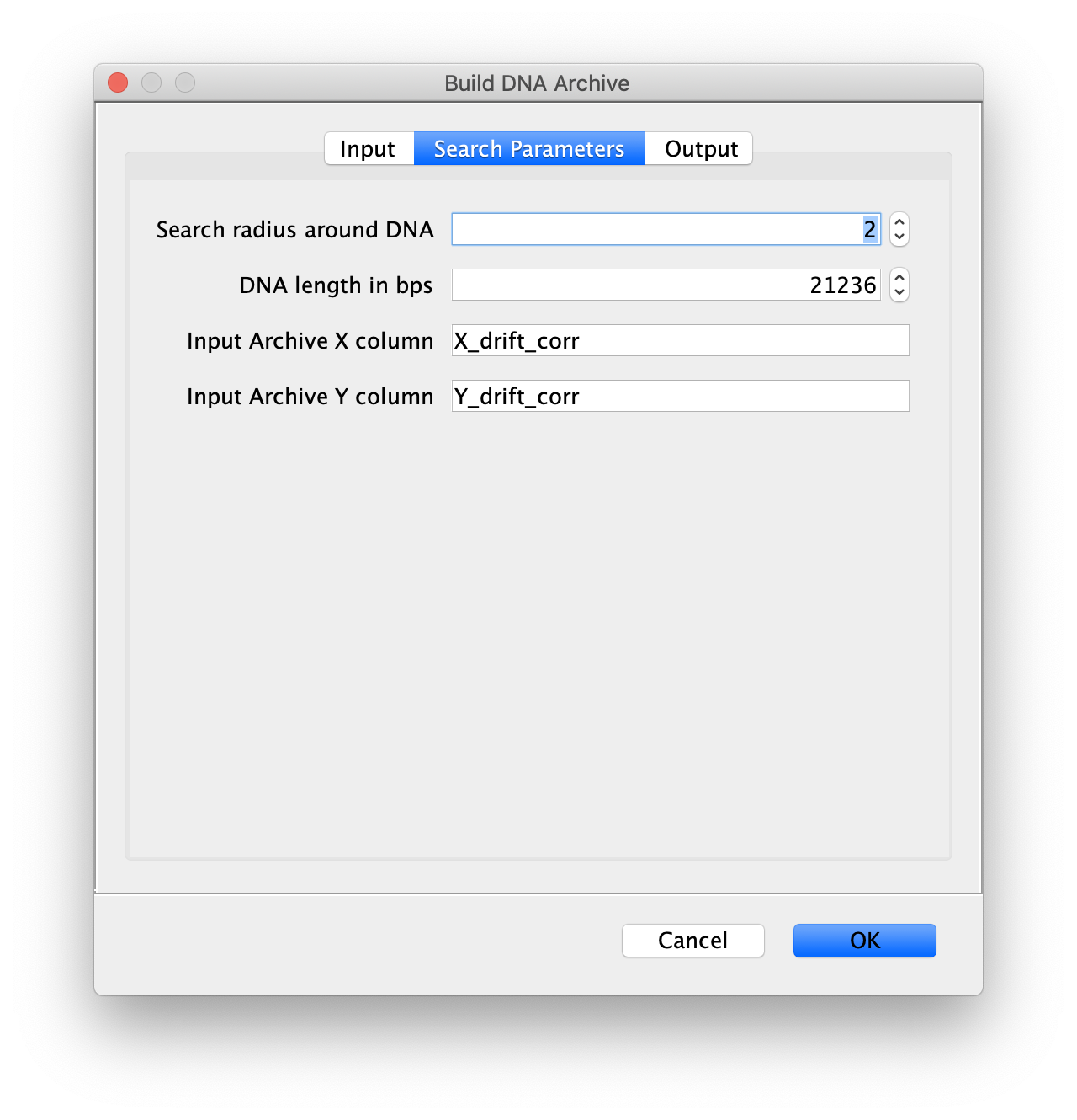
Now all coordinates have been corrected and artefacts have been removed, the DNA location data can be merged with the protein tracking information stored in the Single Molecule Archive. This is done using the build DNA archive command (Plugins>Mars>Molecule>Build DNA Archive) with the settings as shown below.

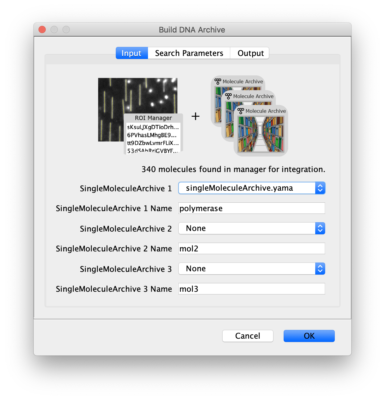
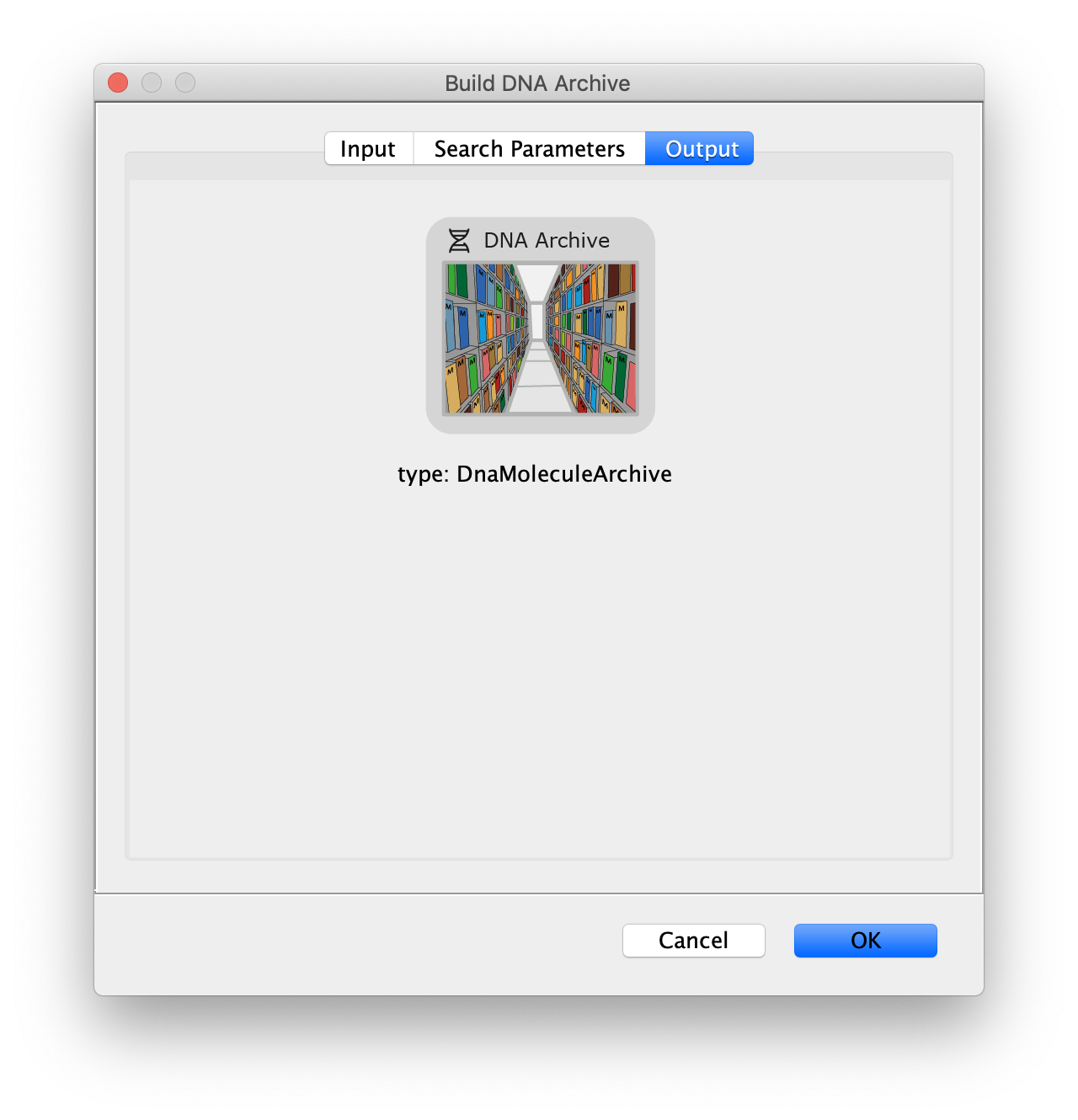
The DNA Molecule Archive should appear containing DNA molecule records that contain tables with all tracked molecules that were found to be located on DNAs as well as their position on DNA and integrated intensity. Now you can see individual tracks of molecules on a specific DNA molecule. You can calculate the speed in bp/s and the exact position on the DNA from the data displayed in the table. Note that some DNA molecules were found to overlap with more than one moving polymerase. These are numbered polymerase1, polymerase2, etc.

Output - Data interpretation

Look at the Molecules in the Video
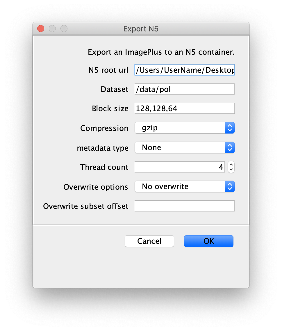
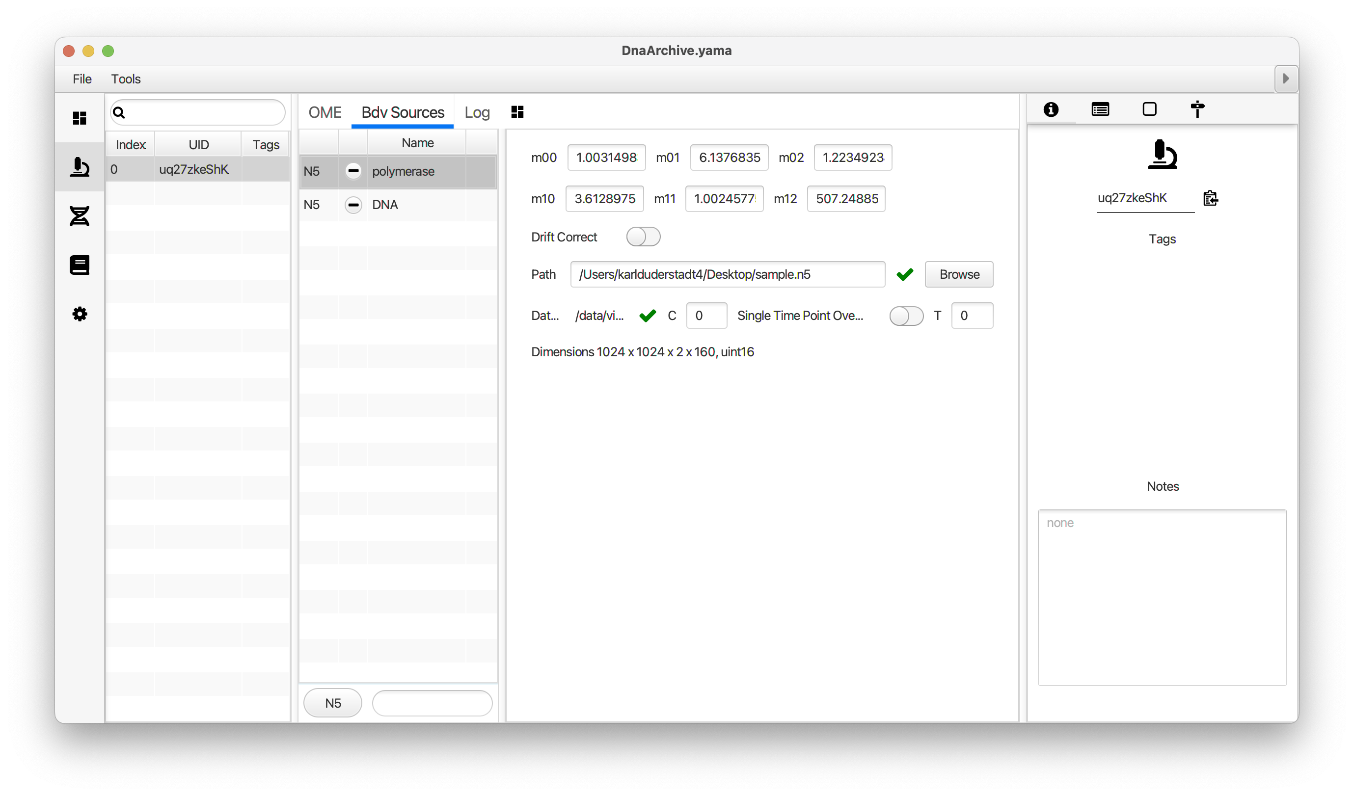
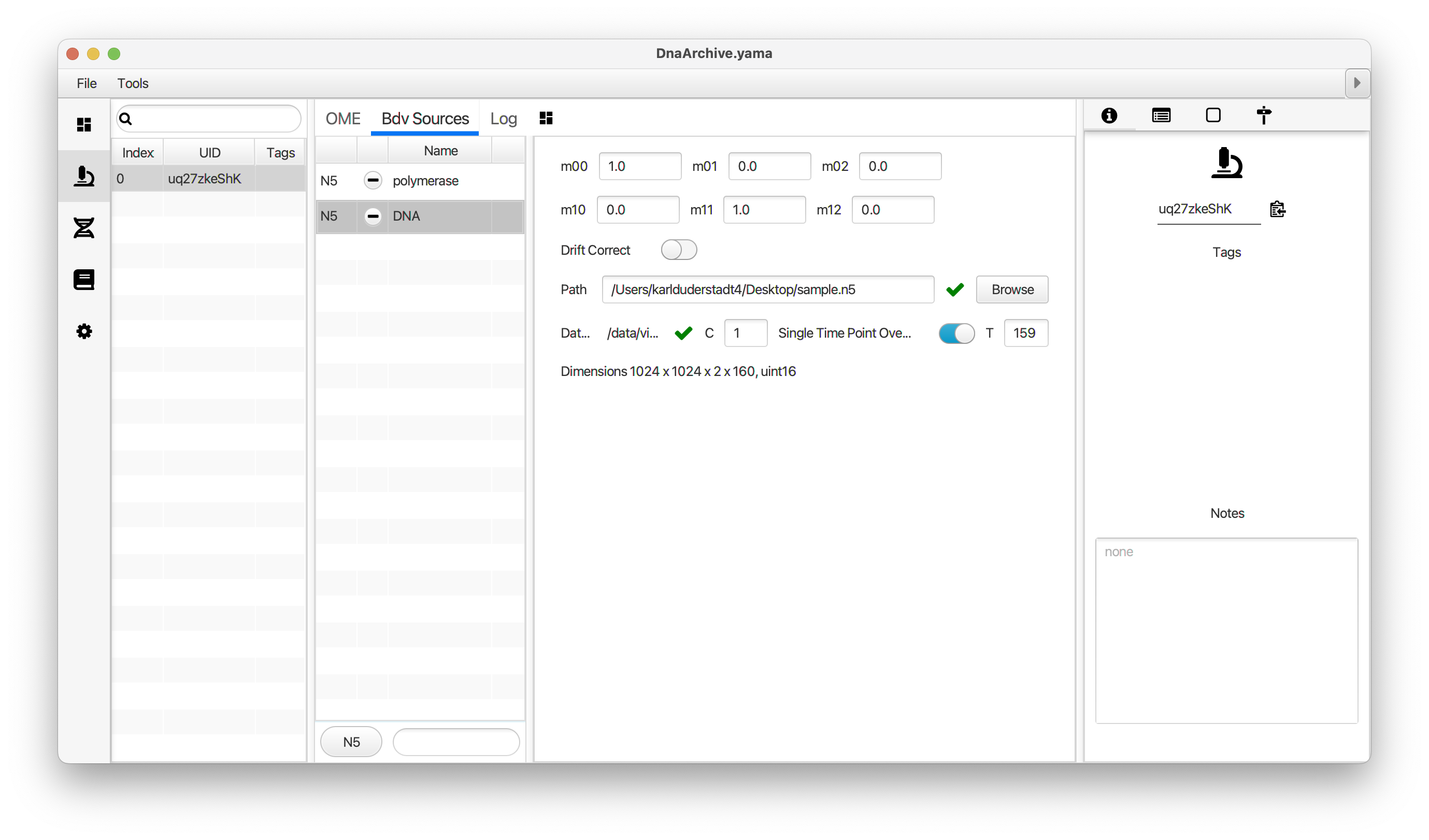
You can use the BigDataViewer in the Mars Rover to look at the molecules in the video. First, convert the video to N5 format (File>Save As>Export N5). The tutorial explains this file conversion and coupling procedure in more detail. Next, add two N5 entries to the BdvSource tab in the metadata tab of the DNA Molecule Archive. In both cases, use the same N5 dataset you just created. The first entry should be called polymerase and be set to C = 0 or channel 0. Also, for the polymerase entry provide the Affine2D conversion matrix parameters as used in the script above, in the line ‘afm.set(…’ and seen below in the window. Make sure to update to your paths, which should give you the green check marks if correct. Next, add a second entry to DNA. In this case use C = 1 or channel 1 and select only time point 159. This will display that single time point all the time for that Source.

Once the entries are correct in the BdvSources tab, open a Bdv window using Tools>Show Video in the DNA Molecule Archive window. This offers the option of opening one or more Bdv views. Open one for this example. This should open a Bdv window with both the polymerase and DNA channels available as sources. Open the settings tab by pressing the small « icon that appears when you hover the mouse over the right edge of the viewer window. This will allow you to choose the colors, contrast min and max as well as other settings. Check the settings below and, most important, change the T, X, and Y to the correct columns for the molecules as below. The checkboxes in the Location tab will highlight molecules in the video using the data in the archive. With rover sync active, the Bdv view will update as you switch between molecule records in the Molecule Archive window. Move through time points (T) by moving the slider on the bottom of the viewer to look at the tracked movement of the protein through the frames.

Kinetic studies
Now that all coordinates with respect to time are calculated for each polymerase that was recorded, many kinetic detailed studies are possible. For example, these include studies of processivity, reaction rate, pausing behavior and studies in presence and absence of other components to understand interactions.

As an example we will examine the global reaction rate of the observed T7 RNA polymerases in our set-up. To do so, we will use the T column as a measure of time, and the ‘Position_on_DNA’ column as a measure of reaction progression since it expresses the position of the protein with respect to the nucleotide position on the DNA. When we now divide the total change in position (progression) by the total time, we obtain the global reaction rate. To do so run the script below in the script editor. Use ‘Groovy’ as the running language.

#@ MoleculeArchive archive

import de.mpg.biochem.mars.molecule.*
import de.mpg.biochem.mars.table.*
import de.mpg.biochem.mars.util.*
import org.scijava.table.*

archive.molecules().forEach{ molecule ->
  MarsTable table = molecule.getTable()
  double ymin = table.min("polymerase_1_Position_on_DNA")
  double ymax = table.max("polymerase_1_Position_on_DNA")
  double Tmin = table.min("polymerase_1_T")
  double Tmax = table.max("polymerase_1_T")
  double dist = ymax - ymin
  double time = Tmax - Tmin
  double speed = dist / time
  molecule.setParameter("dist_DNA",dist)
  molecule.setParameter("del_T",time)
  molecule.setParameter("reaction_rate",speed)
 }

The script above calculates three parameters:

dist_DNA: the total distance the polymerase travelled on the DNA (nucleotides)
del_T: the total time elapsed for this movement (/frame)
reaction_rate: the global reaction rate expressed as nucleotides/frame

These parameter values can be found in the parameter tab.

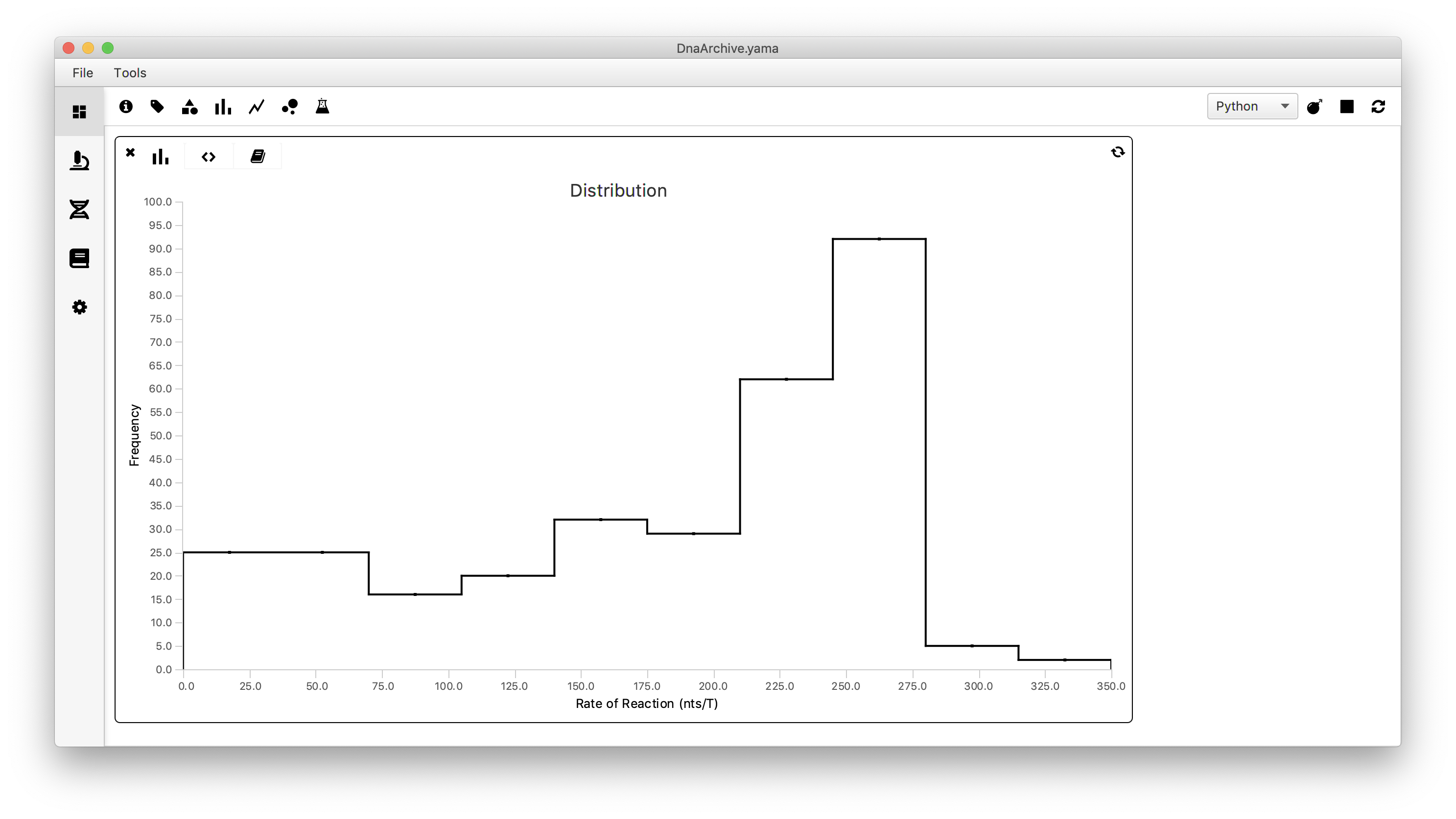
To visualize the spread in the calculated global reaction rate between all measured molecules we will make a plot using a scriptable widget. To do so move to the Dashboard and click the histogram icon. Move to the scripting tab (<>) and past the following code. Select ‘Jython’ as running language and press the refresh button. Then move to the graph tab and obtain the histogram as shown below.

Note: the Dashboard also supports Groovy and Python (PyImageJ). Python (PyImageJ), which we are currently beta testing, allows users to run normal Python 3 scripts when Fiji is launch from a Conda Python environment. We have written a library that will launch Fiji in this way available on conda forage called marspylib. Follow the direction in the readme to set this up and make a comment on the forum if you have problems.

#@ MoleculeArchive archive
#@OUTPUT String xlabel
#@OUTPUT String ylabel
#@OUTPUT String title
#@OUTPUT Integer bins
#@OUTPUT Double xmin
#@OUTPUT Double xmax
#@OUTPUT Double ymin
#@OUTPUT Double ymax

# Set global outputs
xlabel = "Rate of Reaction (nts/T)"
ylabel = "Frequency"
title = "Distribution"
bins = 10
xmin = 0.0
xmax = 350.0
ymin = 0.0
ymax = 100.0

# Series 1 Outputs
#@OUTPUT Double[] series1_values
#@OUTPUT String series1_strokeColor
#@OUTPUT Integer series1_strokeWidth

series1_strokeColor = "black"
series1_strokeWidth = 2

series1_values = []

for molecule in archive.molecules().iterator():
    series1_values.append(molecule.getParameter("reaction_rate"))

Conclusion

You have now successfully analyzed a full dataset containing stretched DNA molecules and a polymerase that moves on this DNA. We deposited a large amount of raw images examining collisions between RNA polymerase an various obstacles including MCMs, ORC, and nucleosomes. This videos can be analyzed using similar workflows. The raw data can be found through the links in the publication.³

References

¹ McAllister W.T. (1997) Transcription by T7 RNA Polymerase. In: Eckstein F., Lilley D.M.J. (eds) Mechanisms of Transcription. Nucleic Acids and Molecular Biology, vol 11. Springer, Berlin, Heidelberg. https://doi.org/10.1007/978-3-642-60691-5_2
² Berg, Jeremy M., John L. Tymoczko, and Lubert Stryer. “Biochemistry.” (2002)
³ Scherr, Wahab, Remus & Duderstadt. (2022). Mobile origin-licensing factors confer resistance to conflicts with RNA polymerase. Cell Reports 38, 110531