Kinetic Changepoint Analysis
level: intermediate, duration: 10-15 min
In this tutorial a kinetic change point analysis is executed. For in-depth information about the algorithms used as well as assumptions the analysis is based on please check the documentation section as well as the paper by F.R. Hill et al1. This tutorial starts with a short introduction to kinetic change points and a discussion about assumptions and continues with a hands-on example using a Molecule Archive.
Introduction
If the kinetic behaviour of a trace changes one calls this a kinetic change point. These changes can be hard to detect since they can be very small and covered by noise. For example on a molecular scale thermal fluctuations are very pronounced which cloak the dynamical behaviour. Extreme changes can be still spotted but the small more subtle changes are hard to detect. The power of single molecule data lays in the detection of these small changes.
An idealized analysis would detect the small changes while not filtering or binning the data and only rely on a small number of user input. Filtering the data would degrade the quality and could lead to loss of information. The same holds true for binning. If the user only gives a small number of inputs the analysis is less biased and is not based on a predefined model. This would also make the analysis more flexible since it can be used for different scenarios. Furthermore, the analysis is more reproducible. The kinetic change point analysis described here and used in this tutorial combines these trades.
Assumptions
The trace should be piece-wise linear between the kinetic change points. It is assumed that the noise is Gaussian distributed. This hold true for biological systems observed with single molecule techniques. Assuming a specific kinetic model is not necessary since that would make it specific for one type of behaviour.
Inputs
-
Position vs. time trajectories: To find the kinetic change points one has to give the position (x, y, z) in which the algorithm should search for the points. Be aware that it depends on the unit of the time axis and the unit of the position which kind of rate you will get (e.g. nm per second).
-
Likelihood ratio/False positive rate: This will help to handle the noise in the data and prevent overfitting of the data
-
Noise level (if it is known): Basically a direct input of the noise which also helps to deal with the noise in the data set.
Output
The analysis will result in the position of kinetic change points and linear fits in between the points. The linear fits contain information about the rate. For example if one would track the position of the replisome over time one would get the rate of replication.
How to: Run the kinetic change point analysis
Open a MoleculeArchive of interest. In case of this tutorial use the archive ‘tutorialvideo_archive.yama’ generated in the Let’s make a Molecule Archive tutorial. Alternatively, one can download this archive on the git repository.
Select the ‘Change Point Finder’ command in the plugin menu (Fiji/Plugins/Mars/KCP/Change Point Finder).
The window shown in the image will open.
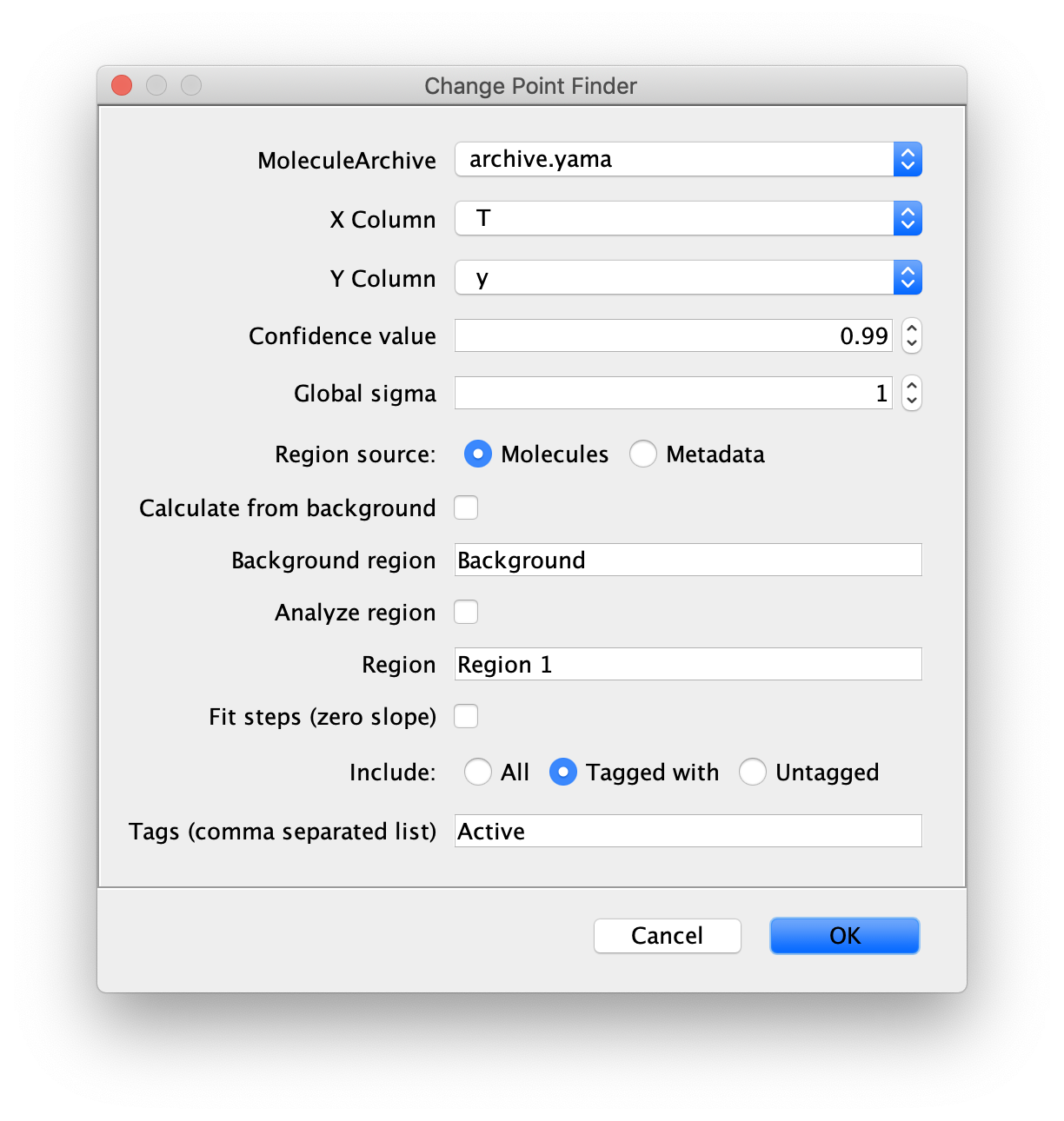
Select the correct Molecule Archive and provide the settings as shown in the image. For a detailed explanation of these settings please visit the documentation.
How to: Read the results of the kinetic change point analysis
The values from the fit can be read out in Mars Rover.
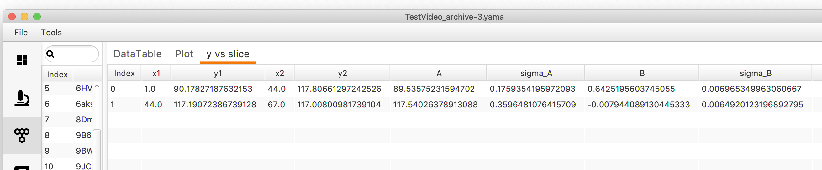
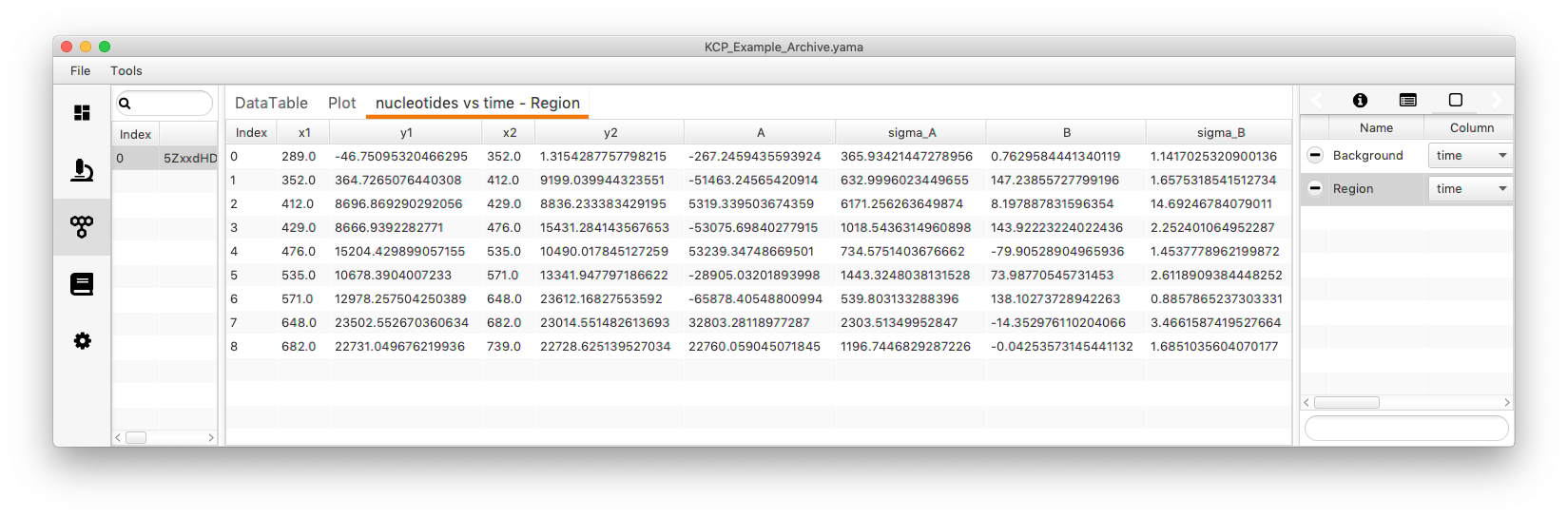
Open “y vs slice”. A table with different columns will appear. “x1” gives the start time and “x2” the end time point of a region where the trace is piece-wise linear. “y1” and “y2” give the corresponding position start and end points. The linear fit between these to points can be described with a line equation (y = Bx + A). The “B” value is the slope of the line which also corresponds to the rate. “A” represents the intercept with the y axis. The sigma values give the standard deviation of either “A” or “B”.
How to: Plot the result of the kinetic change point analysis
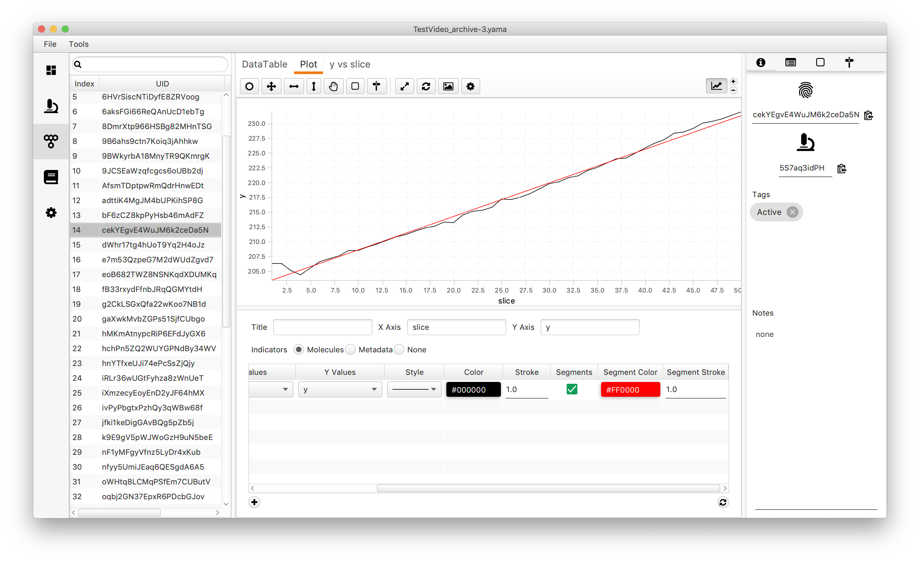
The result from the analysis can be plotted for visual inspection of the fit. Go to the menu of the plot and select “Segments”. After refreshing the plot straight lines which connect the kinetic change points will appear (the color can be adjusted by changing the “Segment color”).
Take it to the next level
By simply looking at the example above one can think that the algorithm produces simple linear regressions. This comes from the fact that most traces in the example only have one transition. To show the real power of the kinetic change point analysis another example is analysed.
The following trace can be found in a separate .yama file in the git tutorials repository named “TestVideo_archive_kcp_complex.yama”. Be aware that the y column is now called “nucleotides” instead.
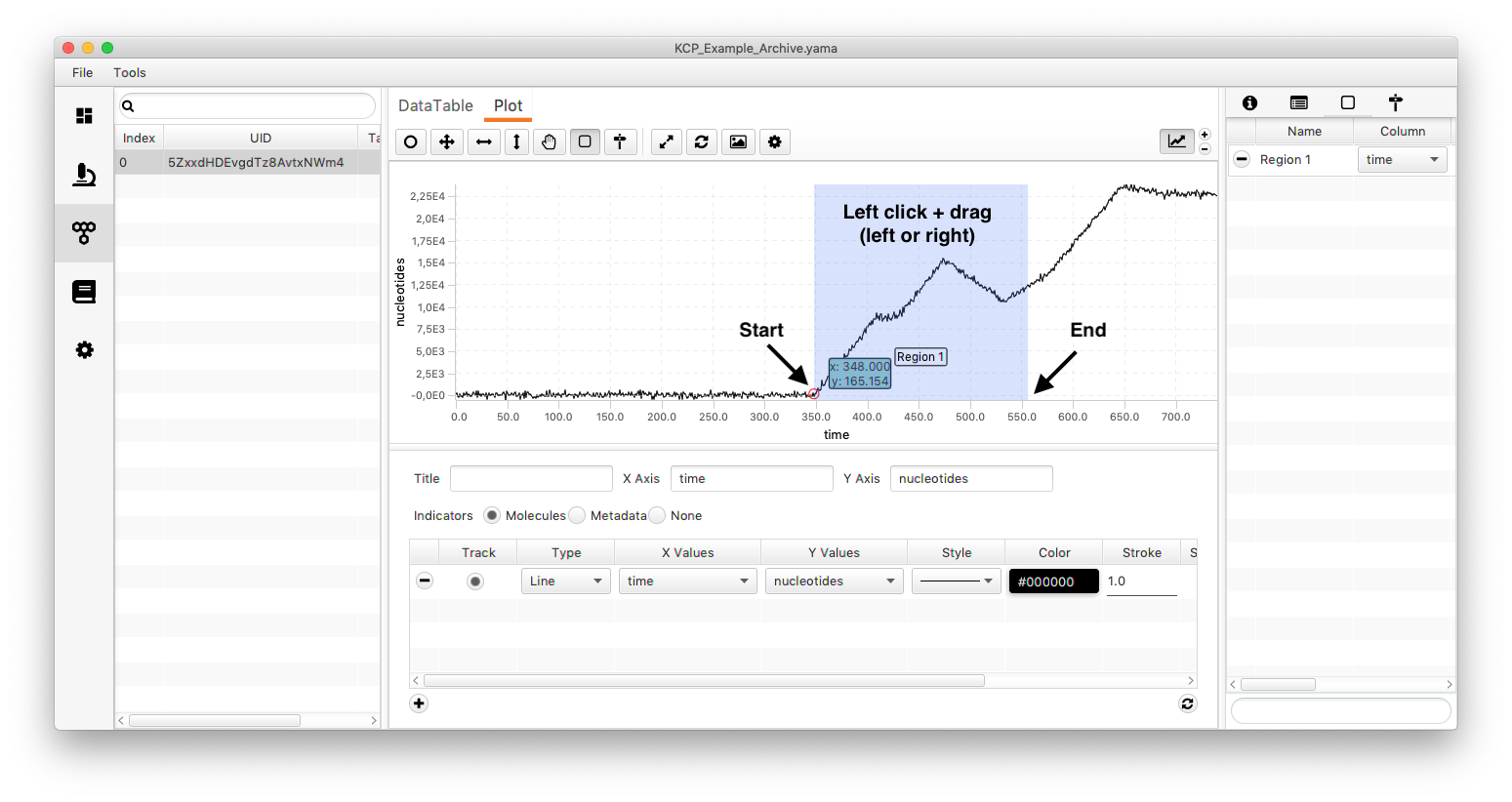
The trace has multiple kinetic changes (see image below). This time an estimation of the background is directly taken from the trace (the global sigma is not considered). For that mark a region and name it background (just for convenience). Then select the region which should be analysed. The trace has simulated gaussian noise.
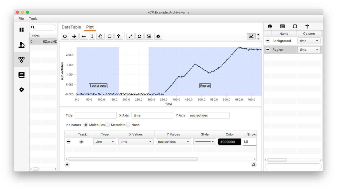
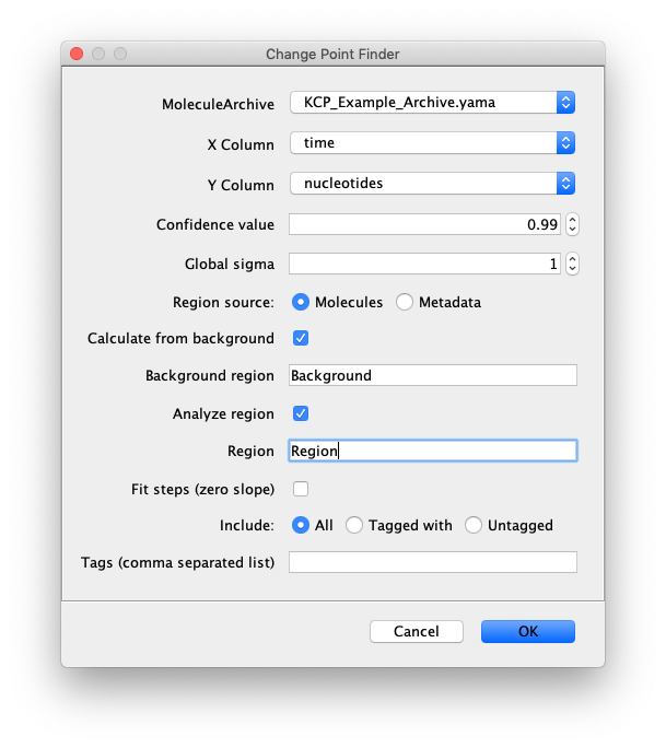
Open the “Change Point Finder” as discussed before. Copy the settings from the window displayed below. By specifying the region of the background the algorithm knows where to check for the background. Same holds true for the region.
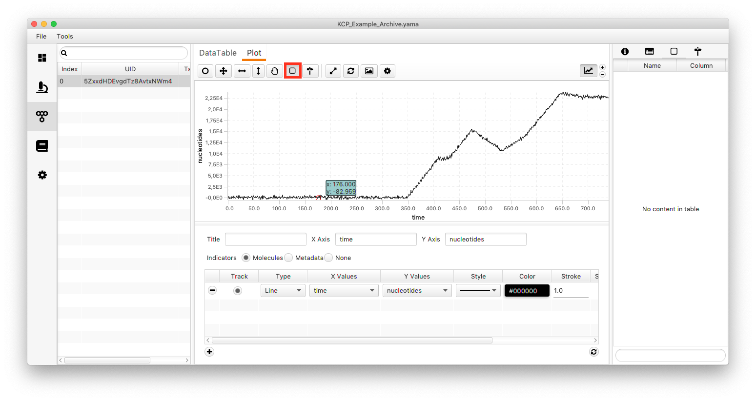
Side note: How are regions created? Select the icon for creating a region (marked in the image below). Move the mouse to the position where the region should start/end and drag the appearing rectangular til the end/start of the region.
After running the analysis one can plot the segments again by checking the box and refreshing the settings. It will now display the different segments in the selected color (in this case red).
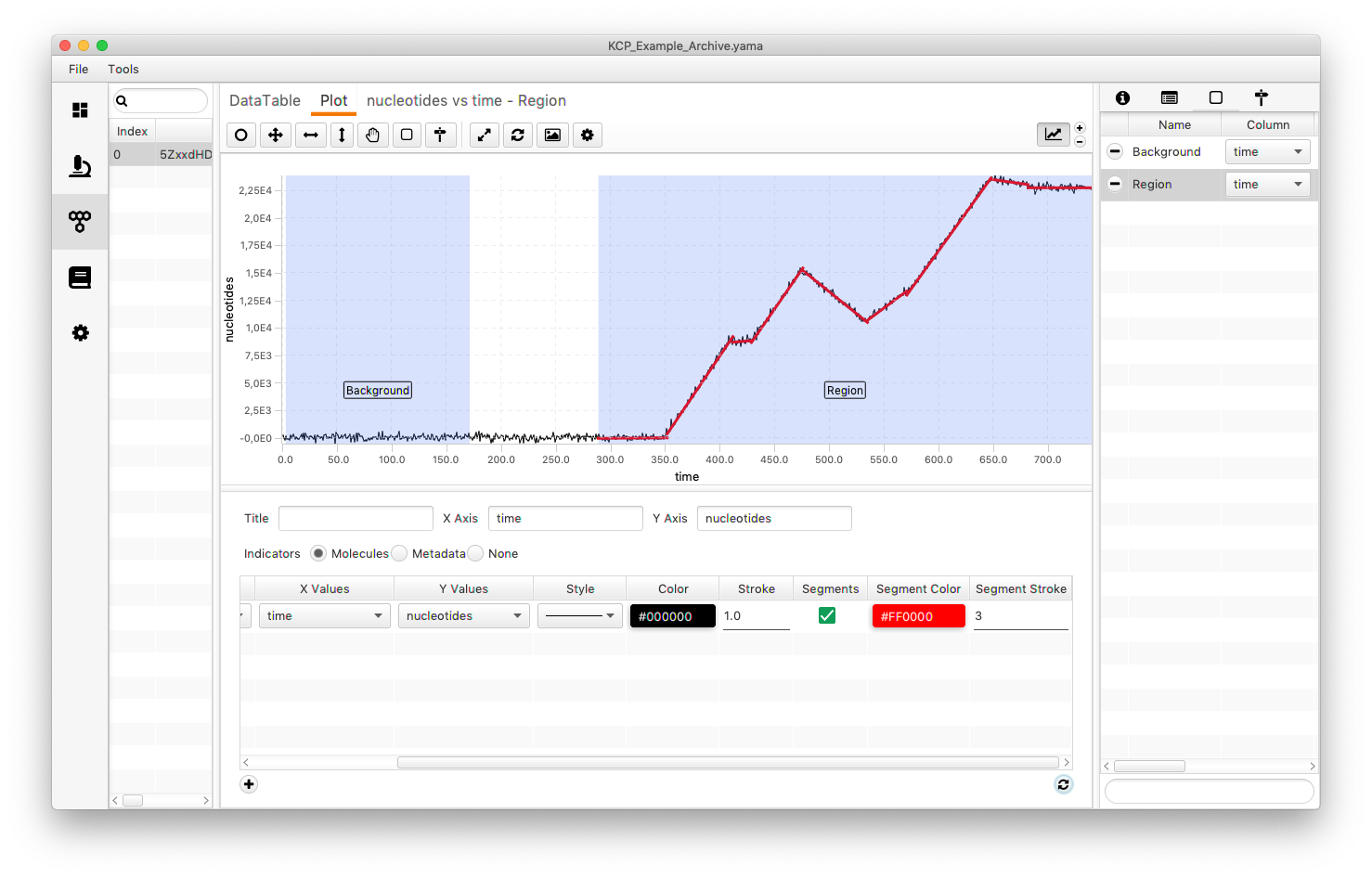
The actual values can be found under “nucleotides vs time - Region”. This tab holding the segment tables is automatically named after the settings. Eight lines with the slope and the intersect are displayed.
1 Hill, F. R., van Oijen, A. M., & Duderstadt, K. E. (2018). Detection of kinetic change points in piece-wise linear single molecule motion. The Journal of Chemical Physics, 148(12), 123317–10. http://doi.org/10.1063/1.5009387