Mars workflow example for dynamic smFRET
This example presents a Mars workflow for the analysis of dynamic smFRET (single-molecule Förster Resonance Energy Transfer) datasets collected using TIRF microscopy. The sample data were collected using a surface-immobilized Holliday junction functionalized with donor and acceptor fluorophores positioned on different DNA arms.1 Imaging was conducted under high Mg2+ concentrations to induce conformational switching of the DNA arms resulting in high and low FRET states.
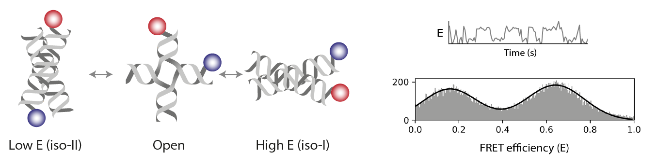
Table of contents
- The FRET Sample Design and Mars Analysis Process
- Data preparation
- Phase I: Locate molecules and integrate fluorescence
- Phase II: Corrections, E calculation, kinetic analysis
- Exploration in Python
- Troubleshooting
- References
The FRET Sample Design and Mars Analysis Process
Dataset Characteristics
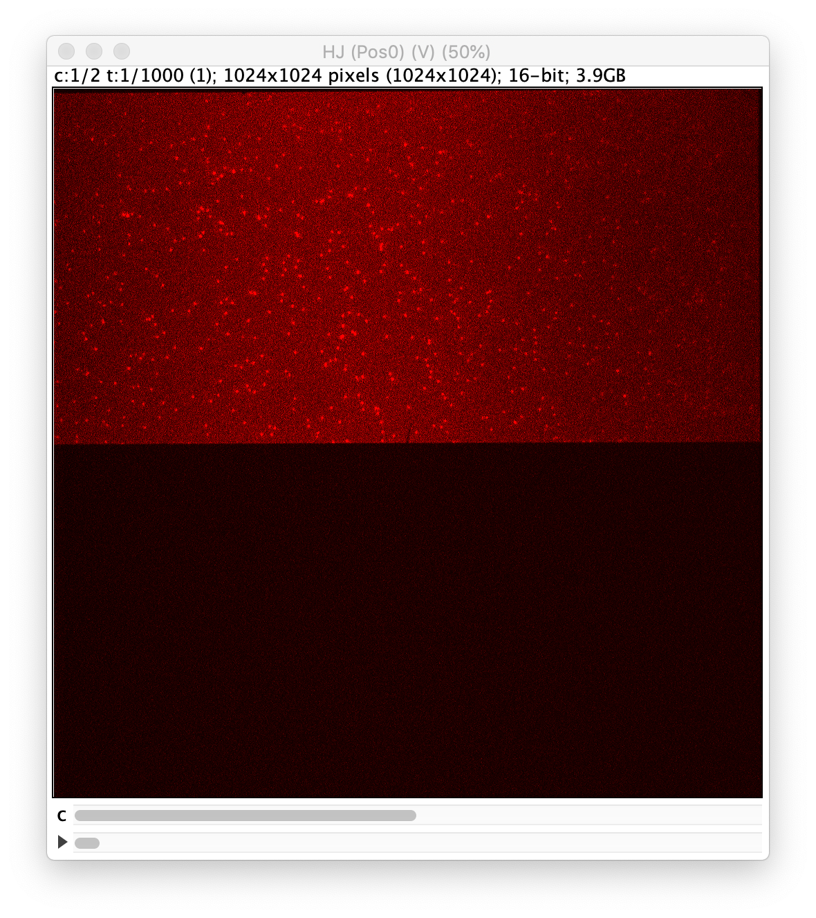
The dataset contains ten separate image sequences each representing a different field of view from the same sample. Imaging was conducted on a micro-mirror TIRF microscope with a dual view using Micro-Manager 2.0. The detection area of the camera is split in half, with each half displaying the signal from a different wavelength. In this way emission can be measured for two wavelengths at the same time and signal correlation is possible. In practice, for this dataset, this means that red emission is collected and shown on the top half, and the green emission on the bottom half of the image (figure 3). Furthermore, the dataset has two channels. One channel for red excitation (C=0) with a 637 nm laser and another for green excitation (C=1) with a 532 nm laser as denoted below by Iemission|excitation. The intensities of peaks are integrated during analysis, used for corrections and the calculation of final E and S distributions.
Comment: Some microscopes are equipped with two cameras and collect FRET images simultaneously by splitting so that the donor signal goes to one camera and acceptor signal to the other. These types of datasets also can be analyzed with this Mars workflow. We suggest combining the videos collected by the two cameras side-by-side into a single artificial dualview. This can be accomplished very easily in Fiji by opening both videos and using the combine command under Image>Stacks>Tools>Combine. This approach depends on the two cameras collecting the same number of images at the same time. Once the two videos are combined into one, this workflow can be followed exactly. This approach also ensures proper registration between the cameras that might not be perfectly aligned with sub-pixel accuracy.
The Analysis Procedure
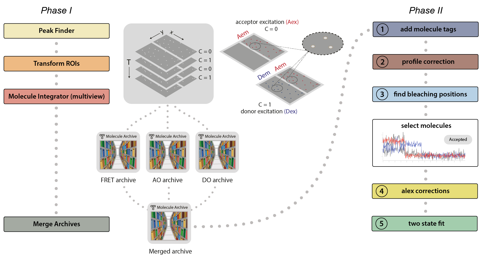
This example was developed in a modular fashion to illustrate how workflows can be built using Mars and to simplify the process of customization for processing other FRET datasets. The workflow has two major phases. In the first phase, displayed below on the left, the emission peaks from the molecules are located and fluorescence intensity is integrated to generate Molecule Archives for donor only (DO), acceptor only (AO), and FRET populations. These are merged into one Molecule Archive that is used in Phase II, displayed on the right, where a sequence of groovy scripts provided in the mars-tutorials repository are used to process the merged Molecule Archive. This includes identification of bleaching positions, scoring intensity traces, and calculating correction factors.
Phase I: Locate molecules and integrate fluorescence
- Identify the peaks (molecule locations) in the top and bottom regions.
- Correlate the peaks in the top and bottom regions to find which molecules have only red emission (acceptor only, AO), only green emission (donor only, DO), or emission from both dyes (FRET).
- Extract the intensity (I) vs. time (T) traces of all molecules and store this information in a Molecule Archive.
- Tag the metadata record of each Molecule Archive with DO, AO, or FRET depending on the molecules selected and integrated.
- Merge all three of the Molecule Archives (DO, AO, and FRET) in preparation for Phase II.
Phase II: Corrections, E and S calculation, kinetic analysis
- Run the FRET workflow 1 add molecule tags groovy script. This script adds the tags on the metadata records (DO, AO, and FRET) to the corresponding molecule records.
- Run the FRET workflow 2 profile correction groovy script. This script corrects for differences in the beam intensity across the field of view.
- Run the FRET workflow 3 find bleaching positions groovy script. This script adds the donor and acceptor bleaching positions (T) to the molecule records. Evaluate the intensity traces and add the Accepted tag to passing molecules.
- Run the FRET workflow 4 alex corrections groovy script. This script calculates all alex correction factors to generate the fully corrected I vs. T traces as well as the FRET efficiency (E) and stoichiometry (S) values.
- Run the FRET workflow 5 two state fit groovy script. This script adds a segments table making the high and low E states based using the threshold provided.
The template for a custom window containing buttons for all the commands and scripts used in the FRET workflows was made using the Fiji ActionBar plugin and is provided in the mars-tutorials repository. Follow the steps in the FRET Power Tools ActionBar tutorial to setup this helpful button window in your local Fiji to simplify and speed up the workflow.
Final distributions and figures are then generated using the dynamic FRET example jupyter notebook provided in the mars-tutorials repository. This notebook requires the file path to the final Molecule Archive generated from the scripts above as input.
Data preparation
Opening the Video
First, download the dataset from Zenodo. To follow along with this example, you will only need Pos0 and the beam_profiles. The analysis procedure for the other fields of view is be the same.
Make sure you have Fiji with Mars installed. Open Fiji and make sure SCIFIO is used by default to open videos (Edit>Options>ImageJ2 tick the use SCIFIO box). Mars comes with a SCIFIO reader for Micro-Manager 2.0 that ensures all metadata is recovered using the Mars image processing commands. Open the video by dragging it from your file explorer to the Fiji bar or using File>Open… and selecting any image in the sequence. The video should look similar to the screenshot in below. If you are trying this workflow with a different video, Mars accepts many other formats including videos opened using BioFormats. However, some metadata may not be recovered and this workflow would require some adaptation if a different collection strategy was used. If you run into trouble or have questions please make a post on the Scientific Community Image Forum with the mars tag.
Affine2D matrix
To correlate the coordinates in the top half of the split view with those of the bottom half of the split view, we use a transformation matrix (Affine2D matrix).
For this dataset, the following matrix will be used:
| Top to bottom matrix | |
|---|---|
| m00 | 1.00276 |
| m01 | 0.000208 |
| m02 | 1.01236 |
| m10 | 0 .000267 |
| m11 | 1.00312 |
| m12 | 507.21025 |
Table 1: Affine2D conversion matrix values. Transforms from the top (acceptor emission) to the bottom (donor emission).
More information about the calculation of this matrix can be found in the Affine2D tutorial
Phase I: Locate molecules and integrate fluorescence
Find and integrate molecules
To calculate all FRET parameters and correction factors three different populations in the sample are of interest: the acceptor only (AO) population, the donor only (DO) population and the FRET population. To facilitate easy data analysis an archive is created for each of these populations separately. These are then later on merged together while ensuring the metadata records for each of these archives is tagged appropriately so molecules are correctly tagged. These tags are used when calculating the correction factors.
All three archives are created following the same workflow: peak identification, ROI transformation to the other halve of the split view, ROI filtering and finally molecule integration to obtain intensity vs. T traces in the Molecule Archive. Below, the workflow to create the FRET archive is shown with screenshots. The procedure is repeated with a few differences described for the creation of the AO and DO Molecule Archives.
The FRET Archive
Find the peaks in the red channel (C=0, top)
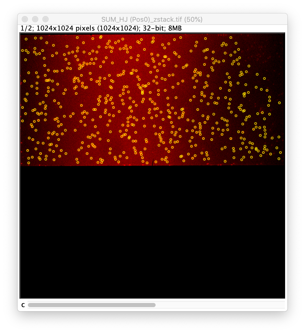
First, for a better fit performance, do a z-projection of the first 10 frames (select average intensity) yielding an average image (Fiji>image>stacks>Z project…). Use this image to find the coordinates of the peaks.
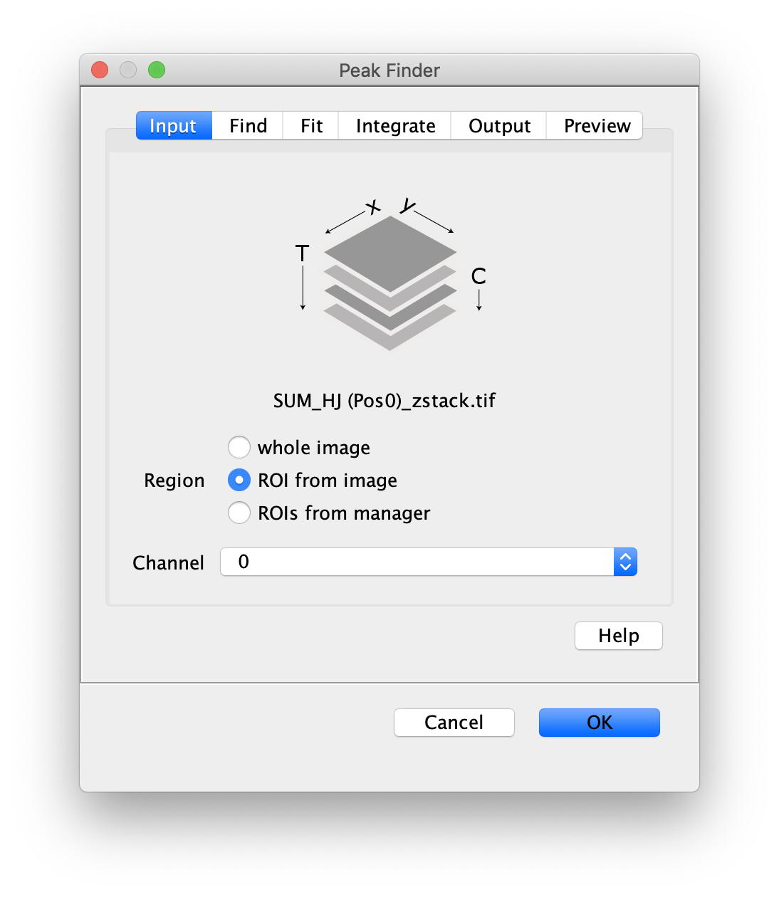
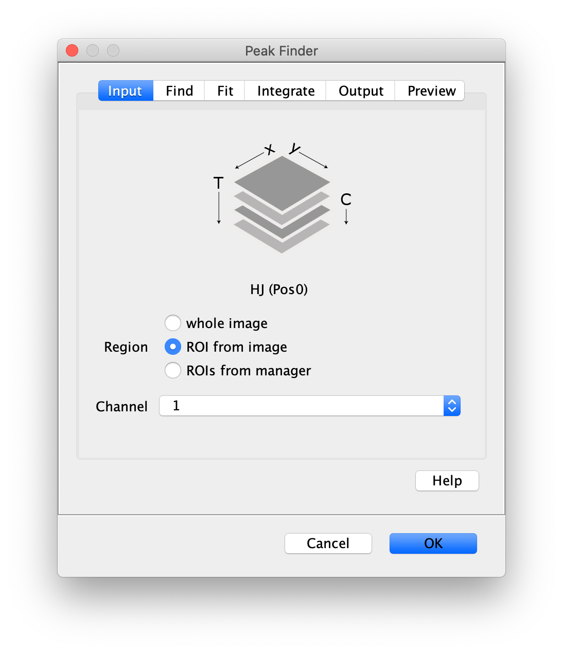
To find the peaks in the top part of the split view in the red channel first select this part of the screen with the box ROI tool and open the Peak Finder (Plugins>Mars>Image>Peak Finder).
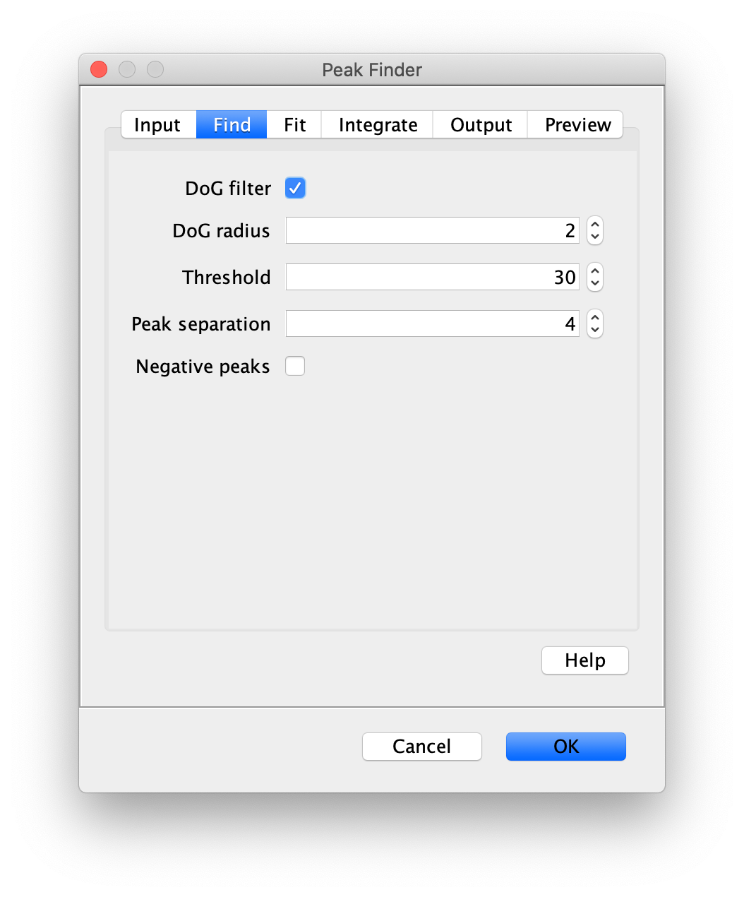
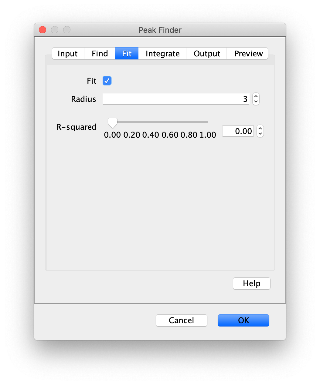
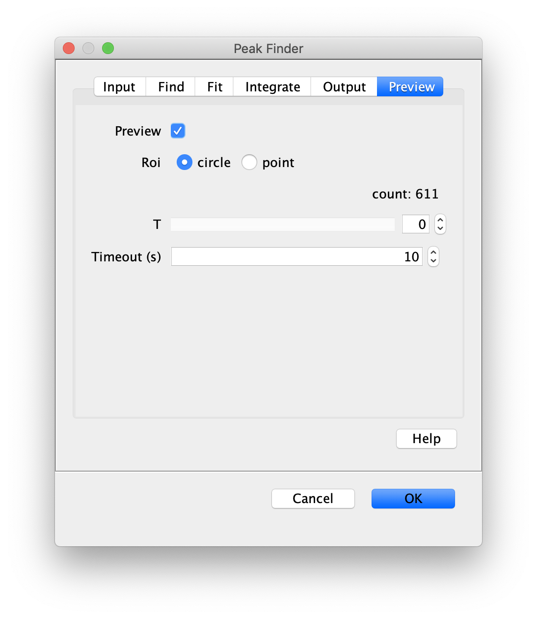
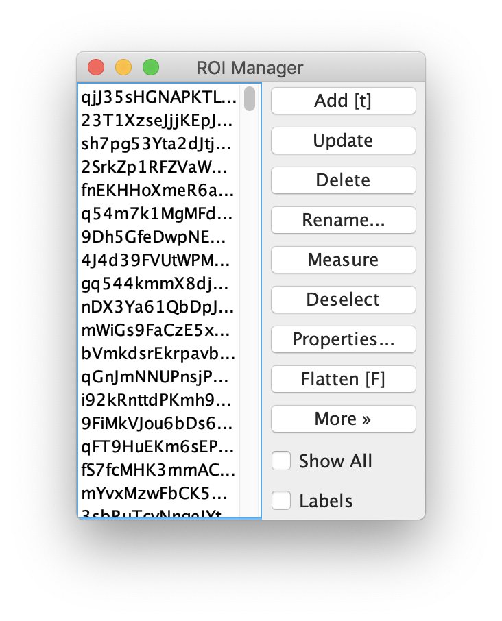
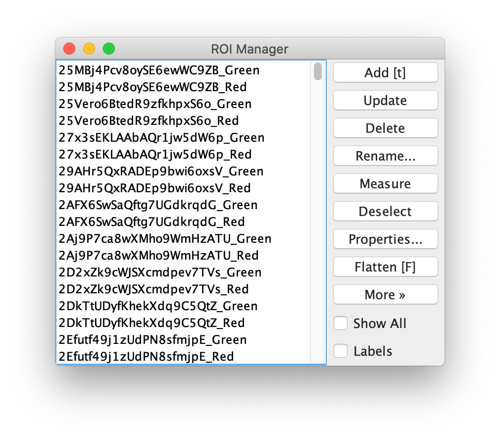
Apply the settings as shown below and check if the peaks are identified correctly by pressing the preview button. If the correct settings are applied the peaks should have an identification marker (circle or point) on them. Press ok to apply the settings and add the ROIs of the identified peaks to the ROI manager. The ROI manager will open and will display the peaks listed by their UID in the manager.
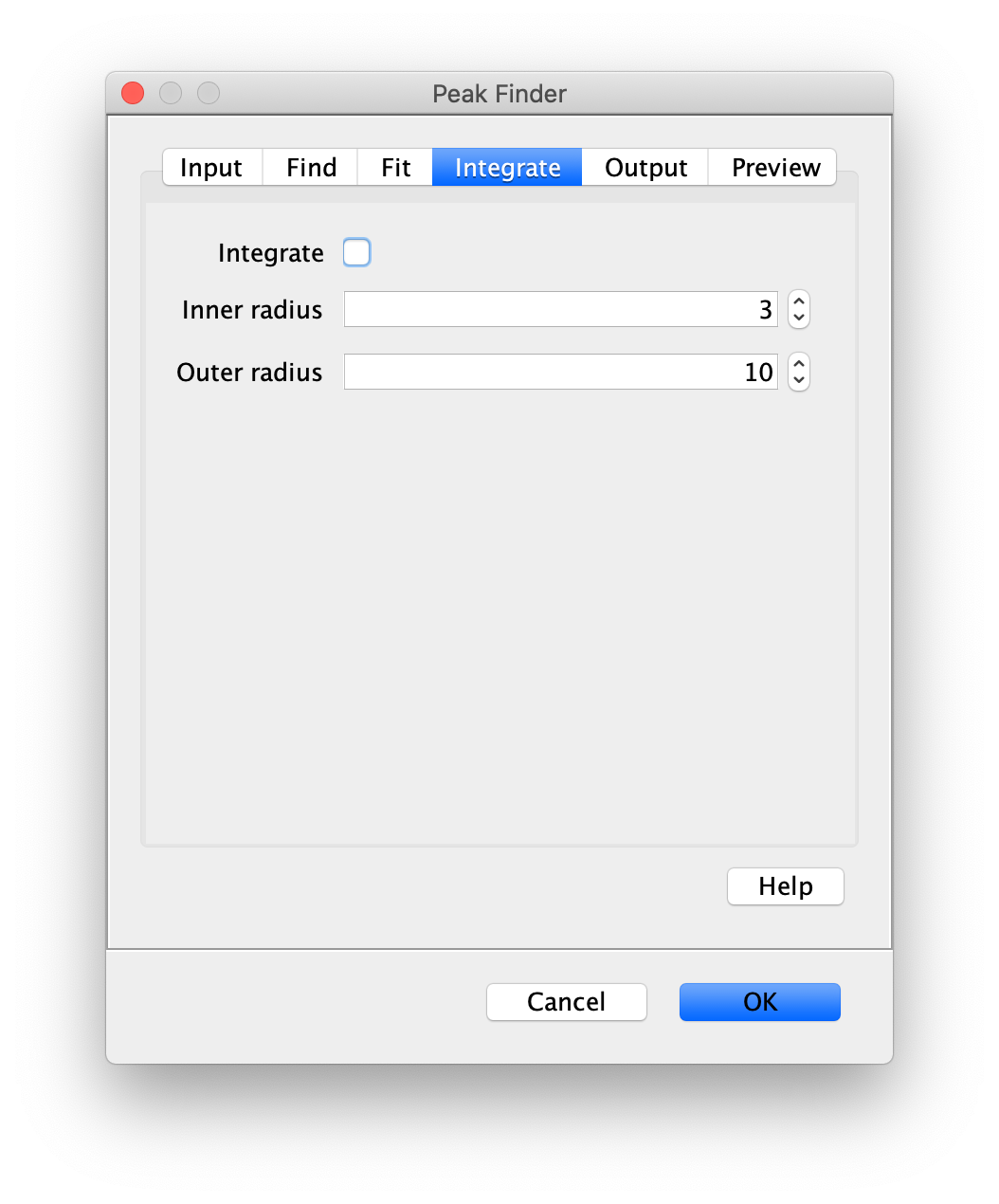
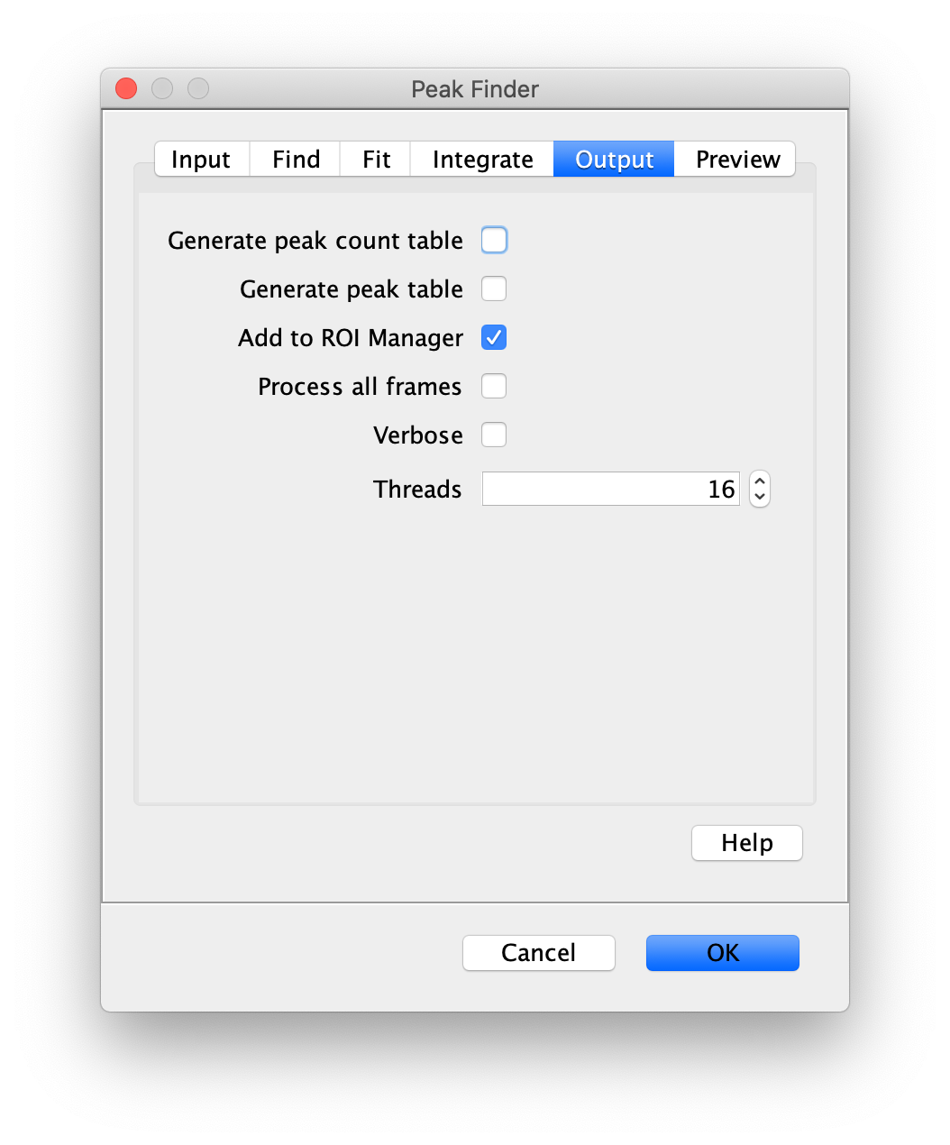
Note: We do not integrate the peaks using the Peak Finder command because this would only provide a table with the currently selected peaks. Instead we will use the Molecule Integrator (multiview) in a later step, which produces a Molecule Archive that contains the integrated signals from all peak populations.
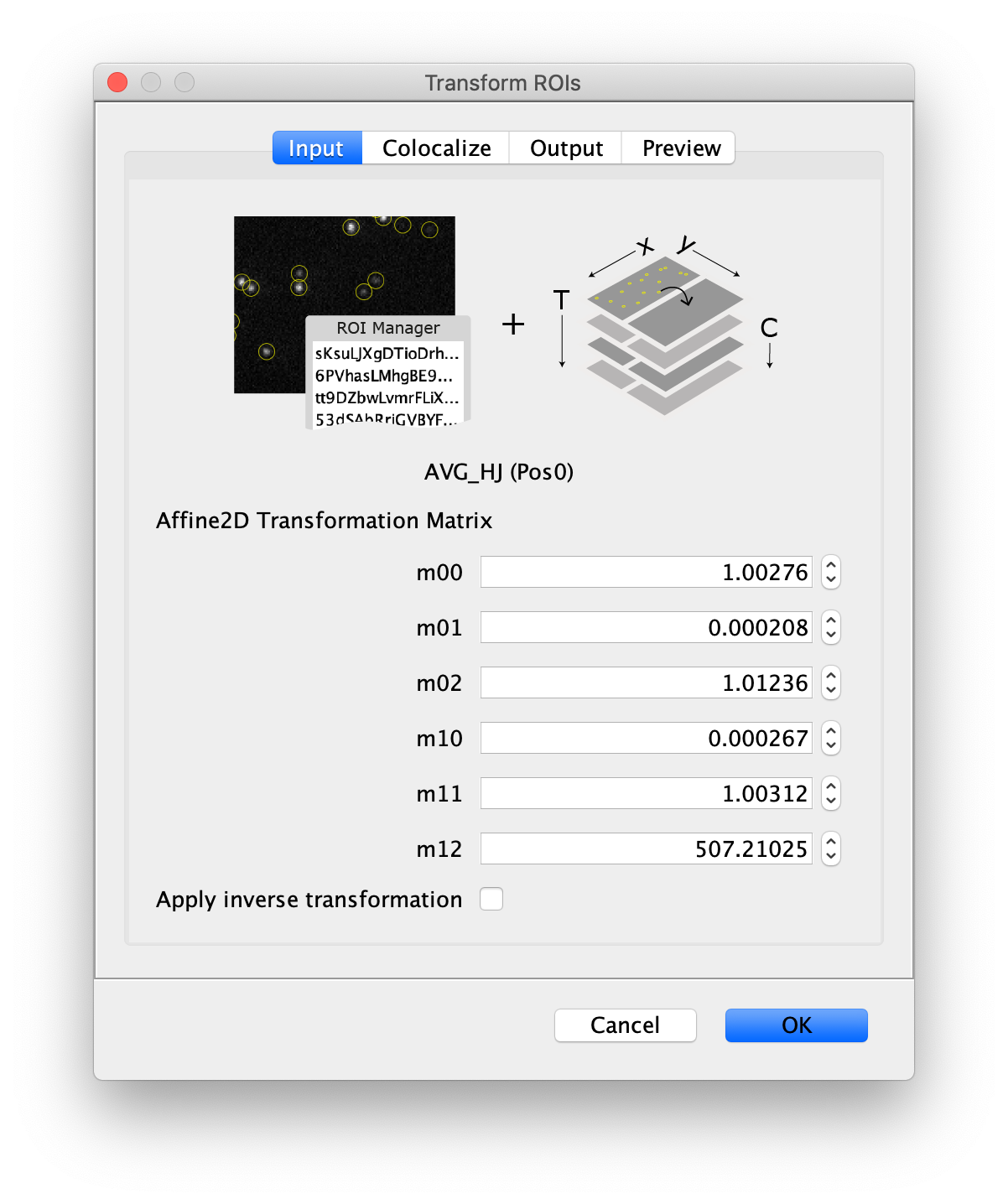
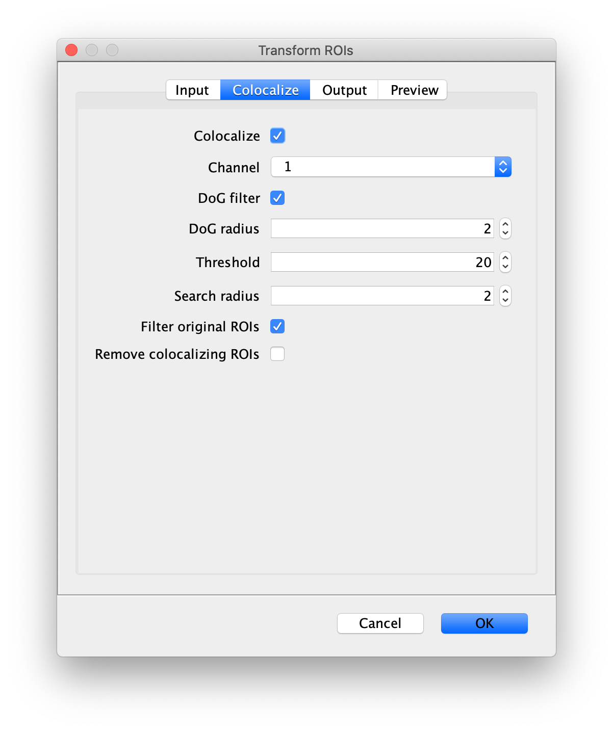
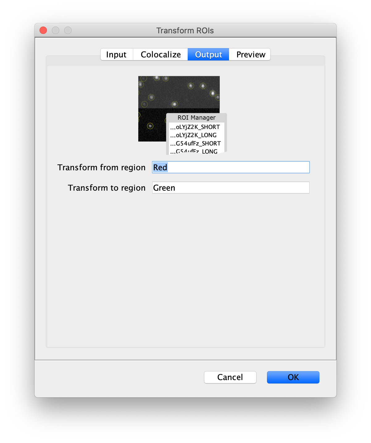
Transform the ROIs to the bottom region of the dual view
Next, transform the peak ROIs to the bottom region of the split view. In this way, in the next analysis step, integration of the peak intensities will be possible at both emission wavelengths at the same time. The transformation is done with the Transform ROIs command (Plugins>Mars>ROI>Transform ROIs). Use the Affine2D matrix as calculated before (see table 1). To ensure we only consider molecules with donor and acceptor signal, we will switch to the FRET channel (C=1) and apply the ‘colocalize’ filter so only peaks that are found in both red and green regions remain. Press ok to add the transformed ROIs to the ROI manager. ROI names will have the format: UID_Red and UID_Green for emission from the same molecule in each region defined in the Output tab of the dialog.
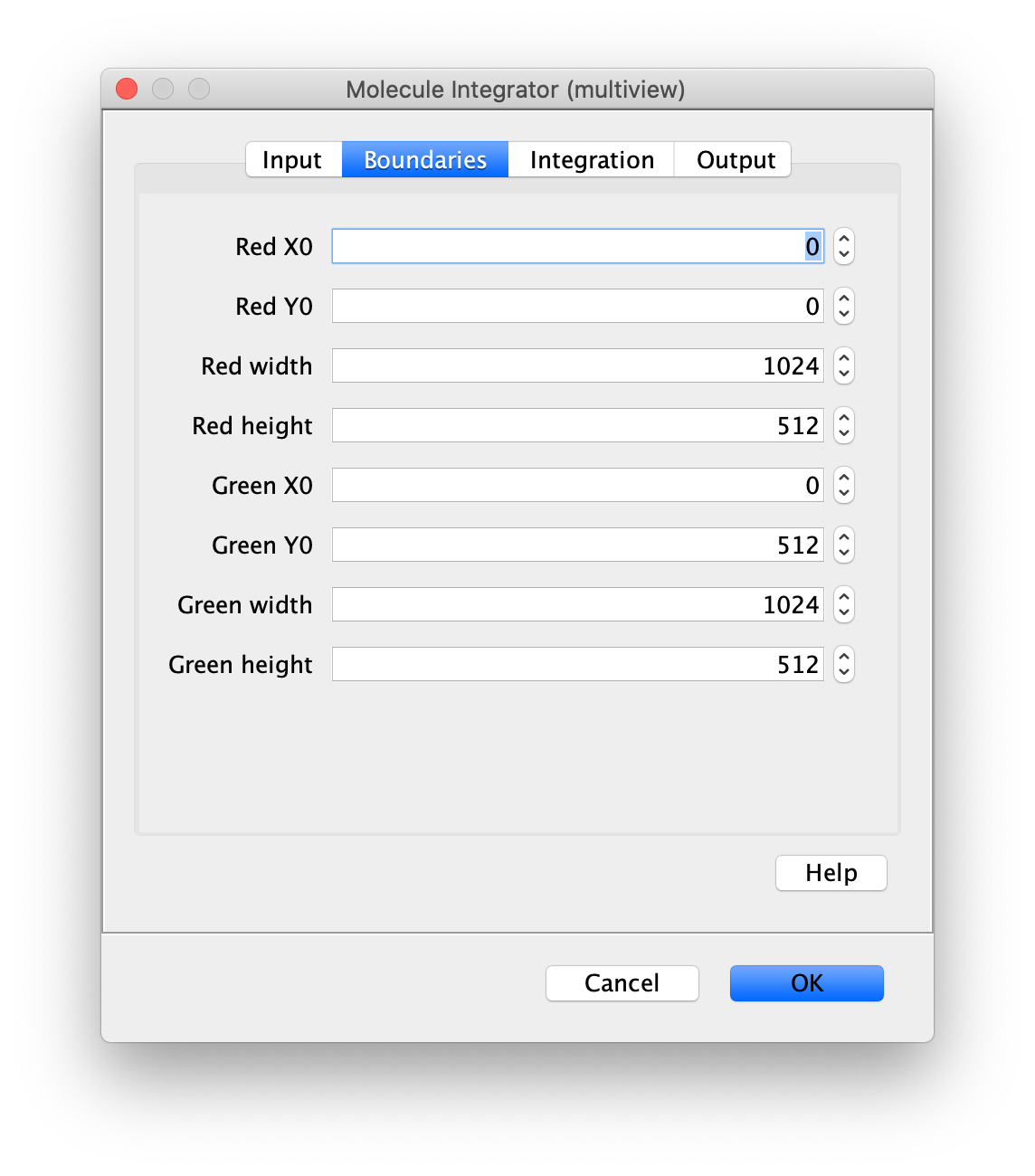
Integrate molecules
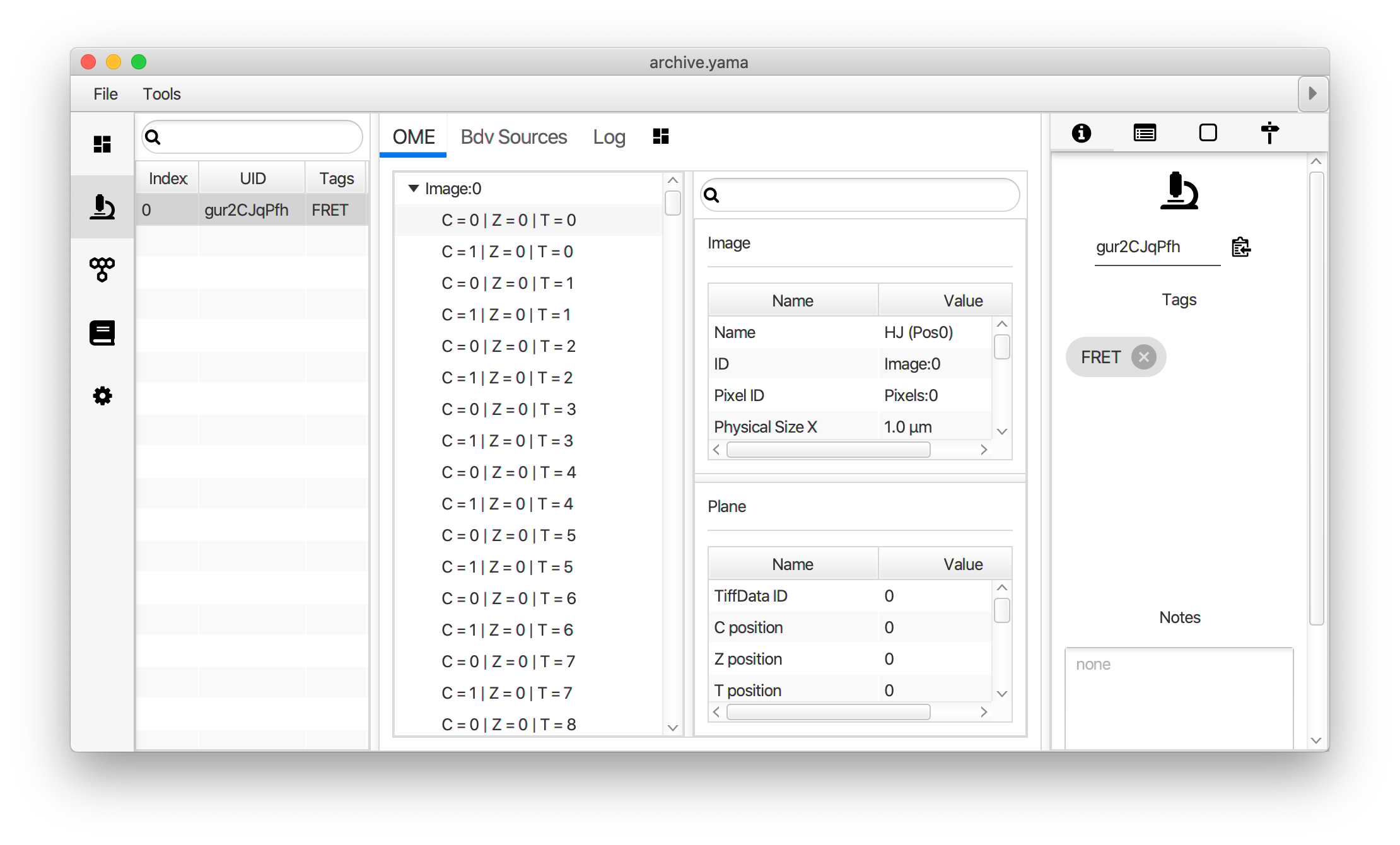
Now switch to the full video (instead of the z projection) by clicking on its window. Then, integrate the peaks using the Molecule Integrator (multiview) command developed for multiview microscopy data (Plugins>Mars>Image>Molecule Integrator (dualview)). Press ok and a Molecule Archive with the results will open automatically upon completion of the calculation. Now the generation of the first archive, the FRET archive, is complete. Select the single metadata record in the Molecule Archive and add the FRET tag. This is required to ensure the population integrated is correctly annotated in the next steps. Save the Molecule Archive with the name FRET_Archive.yama.
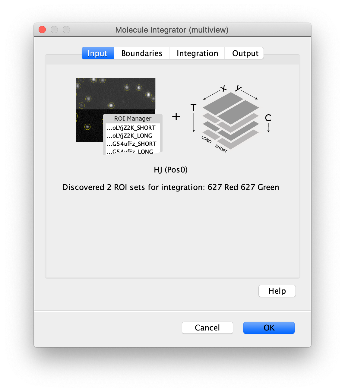
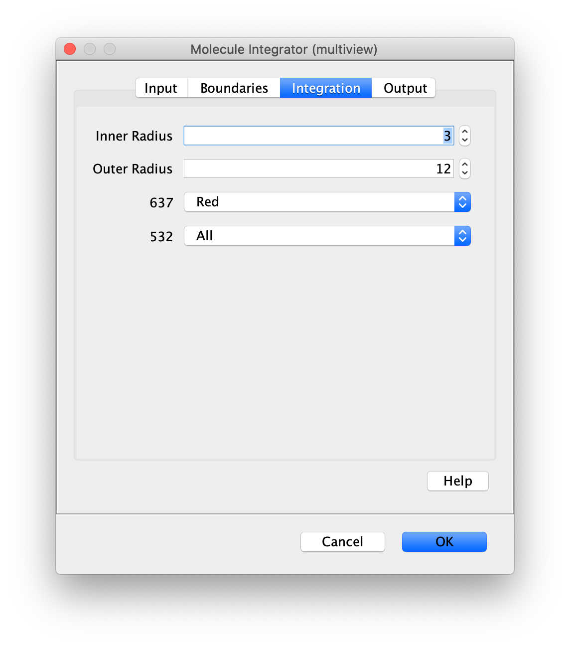

The Molecule Integrator (multiview) command names the fluorescence intensity columns found in the table of each molecule record based on the channel (excitation) and region (emission) names with the format: channel_region. The region names used are specified in the Output tab of the Transform ROIs dialog. The channel names are taken from the video metadata. For the sample data C=0 was named 637 and C=1 was named 532 for the excitation wavelengths used. If no channel names are found in the metadata, the channel indexes will be used as the names (0, 1, etc.).
| Intensity parameter | Name in Mars |
|---|---|
| Iaemaex | “637_Red” (corresponding to C=0, 637 excitation, Red emission) |
| Iaemdex | “532_Red” (corresponding to C=1, 532 excitation, Red emission) |
| Idemdex | “532_Green” (corresponding to C=1, 532 excitation, Green emission) |
Table 2: Overview of definitions of intensity values with their corresponding names in the Molecule Archive.
The AO Archive
First, make sure to clear all entries from the ROI Manager using the Delete button with no ROI selected. This will ensure the new collection of AO ROIs are not added to the previous set of ROIs used for FRET. To create the acceptor only (AO) Archive, follow the same procedure as outlined in section ‘The FRET Archive’ with the only difference being that in this case colocalizing peaks should be filtered out. This is done by checking the ‘Remove colocalizing ROIs’ in the Transform ROIs dialog under the Colocalize tab.
Tag the single metadata record in the resulting Molecule Archive with AO and save it with the name AO_Archive.yama.
The DO Archive
First, make sure to clear all entries from the ROI Manager using the Delete button with no ROI selected. This will ensure the new collection of DO ROIs are not added to the previous set of ROIs used for AO. To create the donor only (DO) Archive, follow the procedure in the section ‘The FRET Archive’ with the following changes:
- Peak Finder: select the lower half of the screen, and select channel 1 in the dialog.
- Transform ROIs: apply the inverse transformation, set channel to 0, check ‘Remove colocalizing ROIs’ and update the region names in the Output tab to reflect a transformation from Green to Red (bottom to top, which is the inverse of what we used when creating the AO and FRET archives).
Tag the single metadata record in the resulting Molecule Archive with DO and save it with the name DO_Archive.yama.
Merge Archives
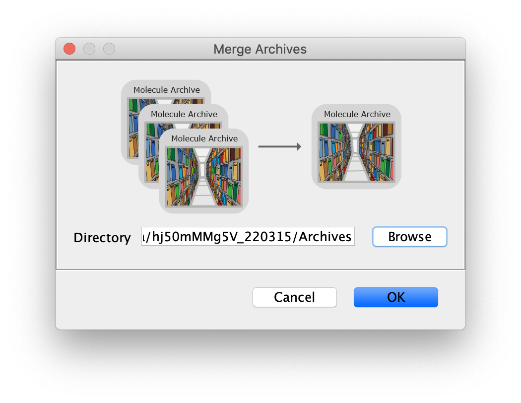
The final step in Phase I is to merge all the archives we created into one. This is required to use the scripts in Phase II that expect AO, DO, and FRET tagged populations. Before merging the archives confirm that the metadata record in each archive is tagged with FRET, AO, or DO consistent with the steps above. If not, make sure to tag them now. All the archives (FRET_Archive.yama, AO_Archive.yama, and DO_Archive.yama) need to be placed in the same folder. Next, use the Merge Archives command (Plugins>Mars>Molecule>Merge Archive) and select the folder. When the command is finished, a merged archive is created that can be found in the same folder (merged.yama). Note: it is very important to save the archives after metadata tagging. Otherwise, the tag will not be in the merged archive and errors will be raised in the subsequent analysis steps.
Phase II: Corrections, E calculation, kinetic analysis
1 add molecule tags
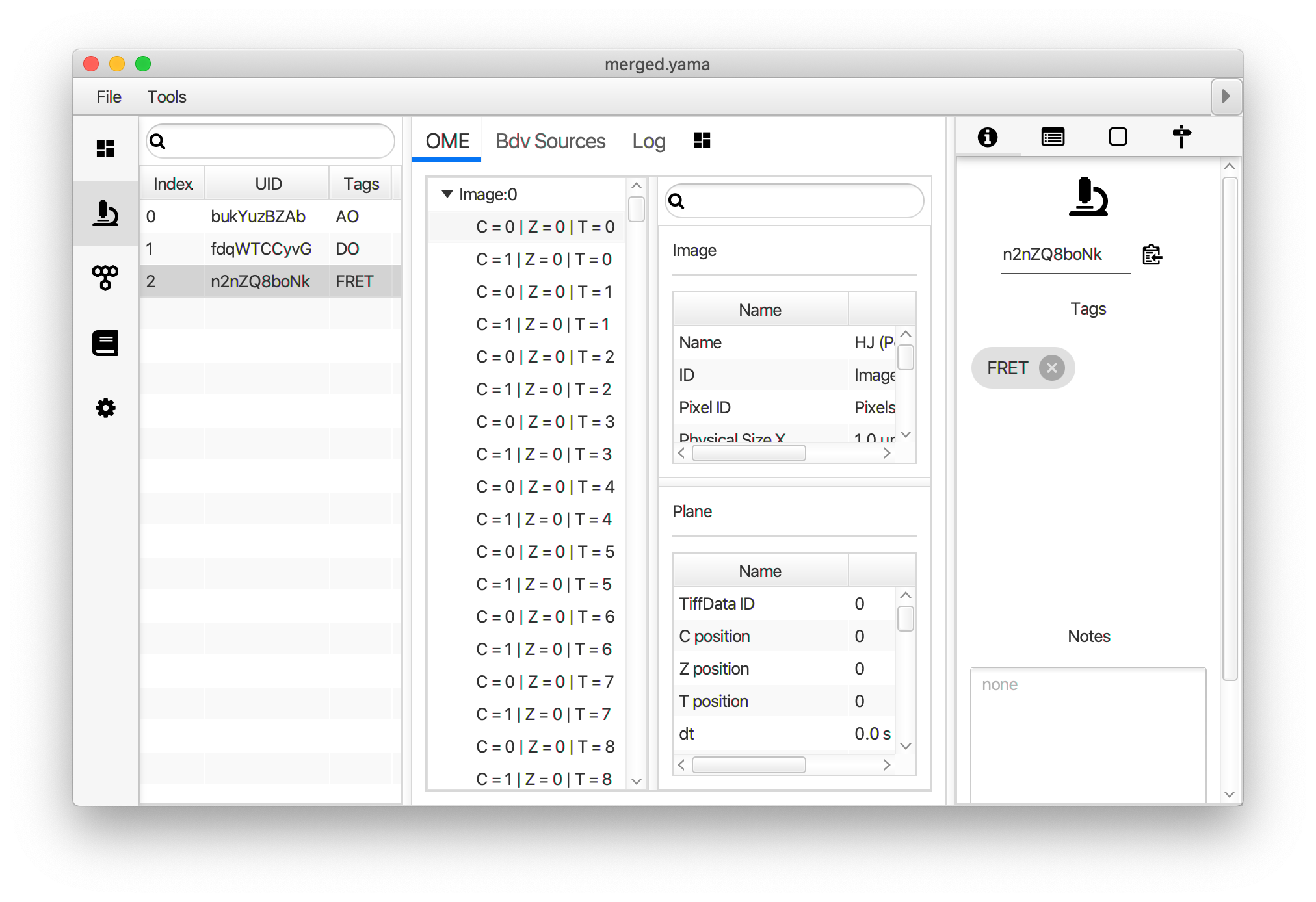
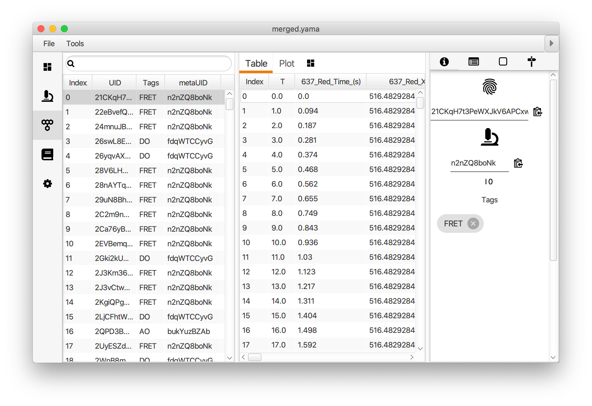
Open the merged Molecule Archive created at the end of Phase I. This should contain three metadata records, one for each archive that was merged and they should have appropriate tags (FRET, AO, or DO). Run the add molecule tags groovy script on the merged Molecule Archive. This script adds the tags on the metadata records to the corresponding molecule records. This can be confirmed by examining the tags on the records in the molecules tab. The rest of the scripts in the workflow require molecule tags.
2 profile correction
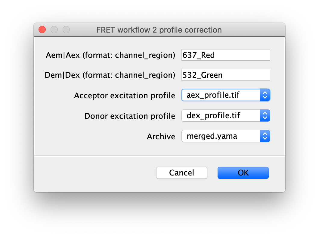
Next run the profile correction groovy script, which corrects for differences in the beam profile intensities across the field of view. This script will take the merged Molecule Archive and the beam profiles included with the sample data as inputs. You will be presented with a dialog when running the script to specify the input files that should already be open in Fiji and the column names for Aem|Aex as well as Dem|Dex. This script will add a new corrected Aem|Aex column with the suffix _Profile_Corrected that will be used in later for in the alex corrections script.
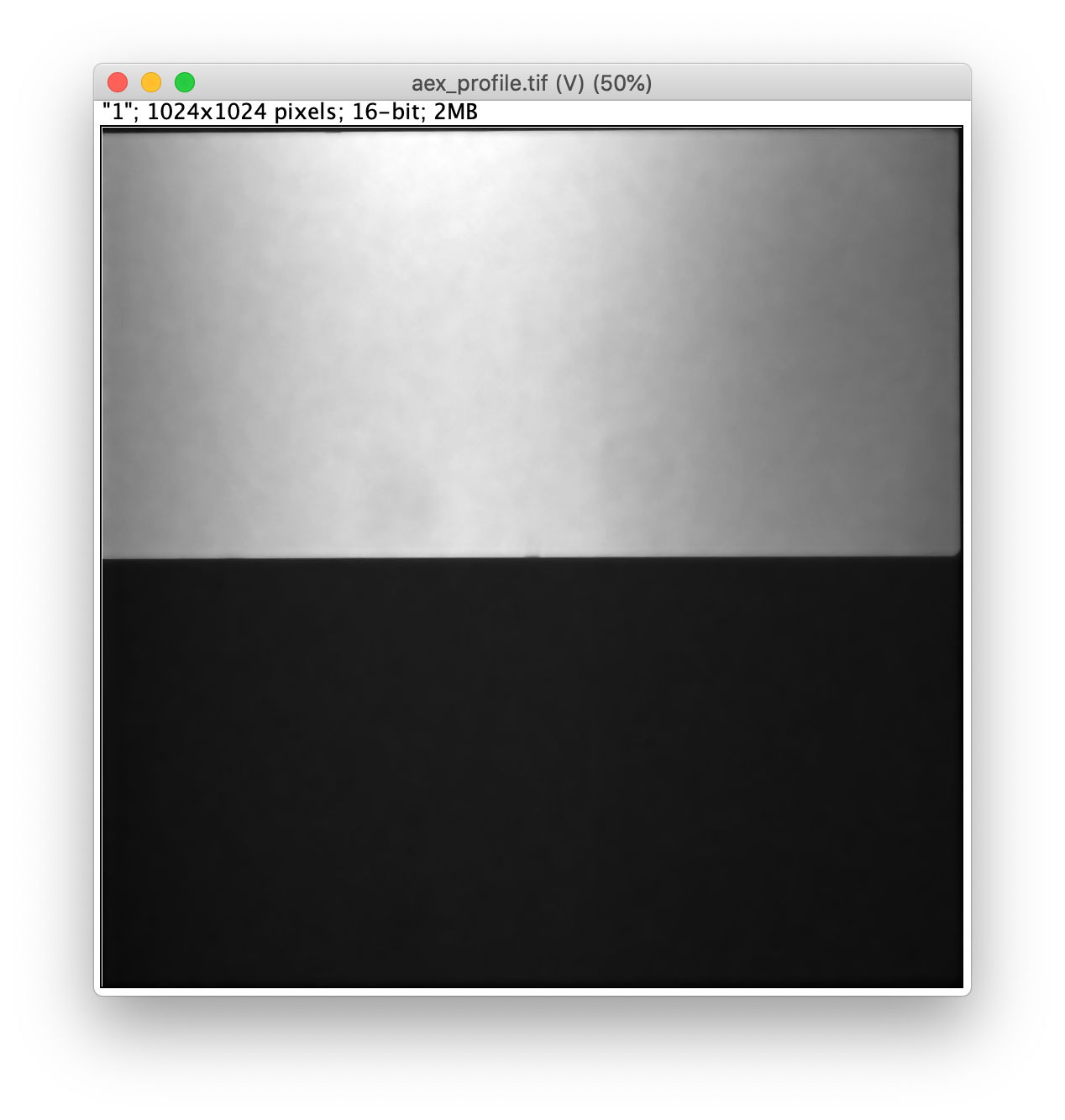
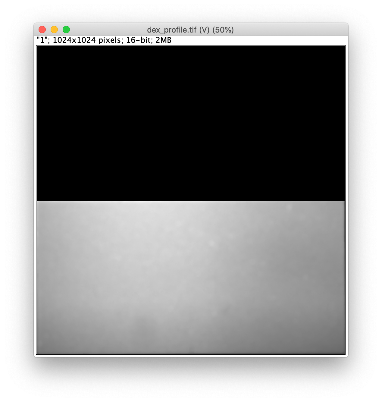
The beam profile correction images were generated using time points at the end of the sample data videos after all dyes bleached (in the range 900 to 1000). The Image>Stacks>Z Project… command was used to generate the mean intensity image from ~10 frames at the end of the video. This mean image was median filtered to remove any remaining features. Images were created for channel 0 (aex_profile) and channel 1 (dex_profile). For the script to work properly the maximum pixel value in the image must be in the region to be corrected. Therefore, the top region of the dex_profile images was deleted to remove remaining crosstalk in the acceptor region. Alternatively, profile images can be created using samples with high dye concentrations.
Warning Make sure to generate the mean intensity image. If you calculate the sum, the max value might become larger than an integer. The script can only handle images with max values that are integers.
3 find bleaching positions
To correctly assess the FRET parameters, it is important to find out the bleaching time points of both dyes and to identify the first dye that bleached. Only the frames of the video up until that point are relevant for FRET. Find the bleaching positions using the find bleaching positions groovy script.
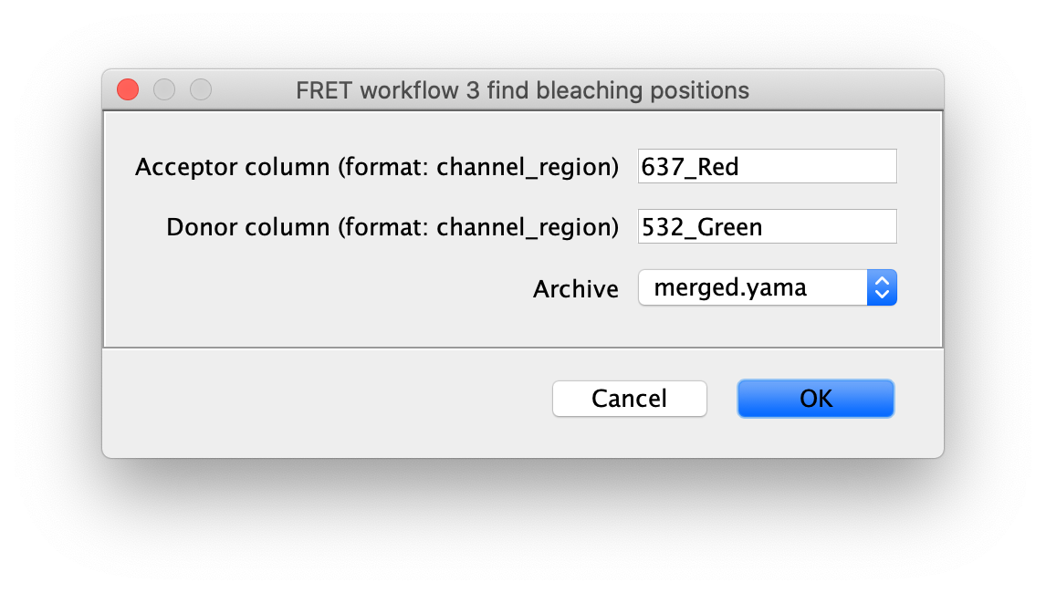
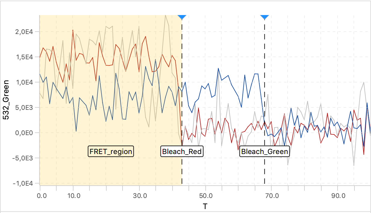
As seen below, this adds the positions Bleach_Red and Bleach_Green to molecule records. To identify the bleaching positions, the script uses the Single Change Point Finder command, which locates the single largest intensity transition within the respective intensity trace. The subsequent scripts only consider the region prior to the first bleach event, highlighted and labeled for clarity below, as the region where FRET occurred.
Plot the traces and add the Accepted tag to passing molecules
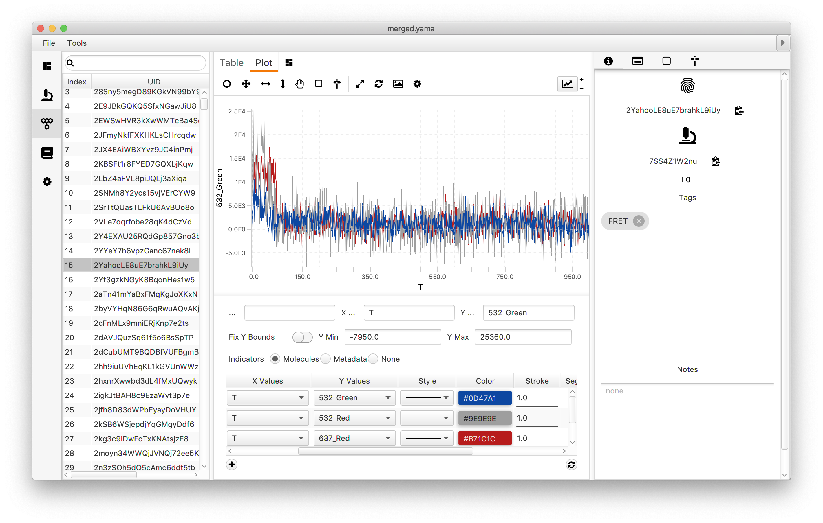
Open the plot sub-tab in the molecules tab and add three line plots representing the three measured intensities (Iaemaex, Idemdex & Iaemdex), if applicable, for each molecule. To do so select the options as shown in the screenshot. The red line represents Iaemaex (AO), the grey line Iaemdex (FRET), and the blue line Idemdex (DO). These are the three intensity vs. time traces that are required for further FRET calculations.
Only molecules marked with the Accepted tag will be used for further analysis. Take care to ensure a consistent set of criteria are applied when marking Accepted molecule records. We used the following criteria for this example:
- There is only 1 donor and only 1 acceptor bleaching step observed in the molecule trace
- Both donor and acceptor are present (in the case of FRET-tagged molecules)
- No major deviations or changes in signal intensity are observed that could indicate an artefact
- The fluorescent signal is significantly higher than the noise of the background
- Donor and acceptor signals are anti-correlated in the FRET region
- There is sufficient FRET life time prior to the first dye bleach event
The selection of suitable AO and DO molecules is equally important to ensure accurate determination of the alpha and delta correction factors that will significantly influence the calculation of beta and gamma. Longer lifetimes, high signal-to-noise, and low background are particularly important. The results of our classification can be directly examined in the holliday_junction_merged.yama and accompanying holliday_junction_merged.yama.rover file final archive for this example that is available from the mars-tutorials repository.
The hot key combinations for molecule tagging can be set in the settings tab of the Molecule Archive. This speeds up the process of tagging significantly. Finally, a validation notebook provided in the mars-tutorials repository offers a report with several measures for the quality of the final set Accepted molecules.
4 alex corrections
Once you have completed the analysis steps above, you are left with a Molecule Archive containing the results from the analysis of Pos0 from the Holliday junction dataset. To increase the number of observations, the workflow above should be repeated for additional positions (fields of view). We repeated the workflow for Pos1, Pos2, and Pos3. We then merged the Molecule Archives from all positions together for further analysis. Determination of accurate correction factors in this step depends on sufficient observations. The $\beta$ and $\gamma$ values in particular will not be accurate for partial datasets.
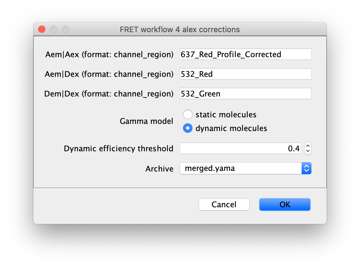
Run the alex corrections groovy script on the Molecule Archive with tagged Accepted molecules. This script calculates all alex correction factors to generate the fully corrected I vs. T traces as well as the FRET efficiency (E) and stoichiometry (S) values and many other outputs described below. There are two options for the model used to calculate the gamma correction, which corrects for differences in excitation and detection factors between donor and acceptor. The ‘dynamic molecules’ model should be used for this dataset.
The ‘dynamic molecules’ model assumes each trace exhibits dynamic switching between FRET states. The efficiency threshold specified will be used to find the mean E and S values for each state used to calculate the gamma correction factor. This script can be re-run multiple times if molecule tags are updated or additional data is merged in.
Comments: The ‘dynamic molecules’ model is also appropriate if more then two states are present. In this case, the threshold value that separates states with the largest differences in E should be chosen. If your molecules do not exhibit dynamic switching between FRET states within individual traces, the ‘static molecules’ gamma model should be used and the threshold E value is not used by the script. This model assumes molecules display different fixed E values. This is illustrated in the static FRET example
The subsections below outline the various corrections performed by the alex corrections groovy script.
Trace-wise background correction
The first correction that is applied to the dataset is a background correction. In this trace-wise process the mean fluorophore intensity after fluorophore bleaching is considered to be the background signal and is subtracted from the calculated fluorophore intensity. This is done for each intensity measurement (Iaemaex, Idemdex & Iaemdex) separately and in a trace-wise manner. The values of the corrected I parameters are stored in the archive as iiIaemaex, iiIdemdex & iiIaemdex respectively. The mean background intensities are stored as molecule parameters (532_Green_Background, 532_Red_Background, and 637_Red_Background).
Correction for leakage ($\alpha$) and direct excitation ($\delta$)
In the next step, two data corrections are carried out: a correction for leakage, the process of donor emission in the acceptor detection channel, and a correction for direct excitation, the process of acceptor emission by direct excitation of the acceptor at the donor wavelength. Both lead to signal intensity distortions when uncorrected and would influence the measured FRET parameters. Therefore they are corrected in this part of the analysis procedure. For more information about these correction parameters the reader is referred to literature9.
The leakage ($\alpha$) and direct excitation ($\delta$) correction factors can be calculated using the formulae below. As indicated, these formulae require the calculated fluorescence intensities from the DO and AO populations respectively. Subsequently, they are implemented in the latter three formulae to find the corrected E and S values. The $\alpha$ and $\delta$ correction factors as well as the calculated FA|D, iiiEapp(DO), and iiiSapp(AO) values will appear as parameters in the archive.
\[\begin{equation} \alpha = \frac{\langle ^{ii}E_{app}^{(DO)} \rangle}{1 - \langle ^{ii}E_{app}^{(DO)} \rangle} \quad\mathrm{and}\quad \delta = \frac{\langle ^{ii}S_{app}^{(AO)} \rangle}{1 - \langle ^{ii}S_{app}^{(AO)} \rangle} \end{equation}\] \[\begin{equation} F_{A|D}=^{ii}I_{Aem|Dex} - \alpha ^{ii}I_{Dem|Dex} - \delta ^{ii}I_{Aem|Aex} \end{equation}\] \[\begin{equation} ^{iii}E_{app} = \frac{F_{A|D}}{F_{A|D} + ^{ii}I_{Dem|Dex}} \quad\mathrm{and}\quad ^{iii}S_{app} = \frac{F_{A|D} + ^{ii}I_{Dem|Dex}}{F_{A|D} + ^{ii}I_{Dem|Dex} + ^{ii}I_{Aem|Aex}} \end{equation}\]Correction for excitation ($\beta$) and detection ($\gamma$) factors
The last data correction step corrects for excitation ($\beta$), normalizing excitation intensities and cross-sections of both acceptor and donor, and detection factors ($\gamma$), normalizing effective fluorescence quantum yields and detection efficiencies of both donor and acceptor. To find both global correction factors a linear regression analysis is performed with the following formula. Note: Each value of iiiEapp and iiiSapp is included in the regression. This means that longer traces have a larger weight in the final fit since these traces contribute a larger number of data points to the dataset used to make a fit.
\[\begin{equation} ^{iii}S_{app}^{(FRET)} = \frac{1}{1 + \gamma * \beta + (1-\gamma)*\beta *^{iii}E_{app}^{(FRET)}} \end{equation}\] \[\begin{equation} \frac{1}{^{iii}S_{app}^{(FRET)}} = 1 + \gamma* \beta + (1-\gamma)*\beta *^{iii}E_{app}^{(FRET)} = b * ^{iii}E_{app}^{(FRET)} + a \end{equation}\]From this equation the dependencies of $\beta$ and $\gamma$ on a and b can be deducted to:
\[\begin{equation} \beta = a + b - 1 \quad\mathrm{and}\quad \gamma = \frac{a - 1}{a + b - 1} \end{equation}\]Once the values of $\beta$ and $\gamma$ have been calculated, the fully corrected E and S values can be calculated. To do so, first FD|D and FA|A are calculated, then added to the archive, followed by the calculation of E and S. Note that these values are extremely sensitive to outliers and will have low significance when used on datasets with a low number of data points.
\[\begin{equation} F_{D|D} = \gamma * ^{ii}I_{Dem|Dex} \quad\mathrm{and}\quad F_{A|A} = \frac{1}{\beta} * ^{ii}I_{Aem|Aex} \end{equation}\] \[\begin{equation} E = \frac{F_{A|D}}{F_{D|D} + F_{A|D}} \quad\mathrm{and}\quad S = \frac{F_{A|D} + F_{D|D}}{F_{D|D} + F_{A|D} + F_{A|A}} \end{equation}\]Molecule table columns
| Molecule table column | Description | Channel | Region | Added by |
|---|---|---|---|---|
| T | OME time points | all | all | Molecule Integrator (multiview) |
| 637_Red_Time_(s) | Time in seconds if discovered in the image metadata | 637 | Red | Molecule Integrator (multiview) |
| 637_Red_X | X coordinate of molecule position | 637 | Red | Molecule Integrator (multiview) |
| 637_Red_Y | Y coordinate of molecule position | 637 | Red | Molecule Integrator (multiview) |
| 637_Red | Local median background corrected integrated intensity | 637 | Red | Molecule Integrator (multiview) |
| 637_Red_Median_Background | Local median background intensity | 637 | Red | Molecule Integrator (multiview) |
| 637_Red_Uncorrected | Raw integrated intensity with no background correction | 637 | Red | Molecule Integrator (multiview) Verbose mode |
| 637_Red_Mean_Background | Local mean background intensity | 637 | Red | Molecule Integrator (multiview) Verbose mode |
| 532_Red_Time_(s) | Time in seconds if discovered in the image metadata | 637 | Red | Molecule Integrator (multiview) |
| 532_Red_X | X coordinate of molecule position | 532 | Red | Molecule Integrator (multiview) |
| 532_Red_Y | Y coordinate of molecule position | 532 | Red | Molecule Integrator (multiview) |
| 532_Red | Local median background corrected integrated intensity | 532 | Red | Molecule Integrator (multiview) |
| 532_Red_Median_Background | Local median background intensity | 532 | Red | Molecule Integrator (multiview) |
| 532_Red_Uncorrected | Raw integrated intensity with no background correction | 532 | Red | Molecule Integrator (multiview) Verbose mode |
| 532_Red_Mean_Background | Local mean background intensity | 532 | Red | Molecule Integrator (multiview) Verbose mode |
| 532_Green_Time_(s) | Time in seconds if discovered in the image metadata | 532 | Green | Molecule Integrator (multiview) |
| 532_Green_X | X coordinate of molecule position | 532 | Green | Molecule Integrator (multiview) |
| 532_Green_Y | Y coordinate of molecule position | 532 | Green | Molecule Integrator (multiview) |
| 532_Green | Local median background corrected integrated intensity | 532 | Green | Molecule Integrator (multiview) |
| 532_Green_Median_Background | Local median background intensity | 532 | Green | Molecule Integrator (multiview) |
| 532_Green_Uncorrected | Raw integrated intensity with no background correction | 532 | Green | Molecule Integrator (multiview) Verbose mode |
| 532_Green_Mean_Background | Local mean background intensity | 532 | Green | Molecule Integrator (multiview) Verbose mode |
| 637_Red_Profile_Corrected | Local median background corrected, beam profile corrected, integrated intensity | 637 | Red | 2 profile correction |
| iiIdemdex | Donor emission after subtracting mean background after photobleaching | 532 | Green | 4 alex corrections |
| iiIaemaex | Acceptor emission after subtracting mean background after photobleaching | 637 | Red | 4 alex corrections |
| iiIaemdex | Acceptor emission from FRET after subtracting mean background after photobleaching | 532 | Red | 4 alex corrections |
| iiEapp | FRET efficiency after correcting for background after photobleaching | - | - | 4 alex corrections |
| iiSapp | Stoichiometry after correcting for background after photobleaching | - | - | 4 alex corrections |
| FAD | Acceptor emission from FRET corrected for background, leakage ($\alpha$), direct excitation ($\delta$) | 532 | Red | 4 alex corrections |
| iiiEapp | FRET efficiency after correcting for background, leakage ($\alpha$), direct excitation ($\delta$) | - | - | 4 alex corrections |
| iiiSapp | Stoichiometry after correcting for background, leakage ($\alpha$), direct excitation ($\delta$) | - | - | 4 alex corrections |
| FDD | Donor emission after correcting for background, excitation ($\beta$) and detection ($\gamma$) factors | 532 | Green | 4 alex corrections |
| FAA | Acceptor emission after correcting for background, excitation ($\beta$) and detection ($\gamma$) factors | 532 | Green | 4 alex corrections |
| SUM_Dex | Sum of acceptor and donor emission during FRET (FAD + FDD). Expected to be stable in FRET region. | - | - | 4 alex corrections |
| SUM_signal | Sum of all dye emissions (FAA + FAD + FDD). Expected to be stable in FRET region. | - | - | 4 alex corrections |
| E | Fully corrected FRET efficiency (background, $\alpha$, $\delta$, $\beta$, $\gamma$) | - | - | 4 alex corrections |
| S | Fully corrected stoichiometry (background, $\alpha$, $\delta$, $\beta$, $\gamma$) | - | - | 4 alex corrections |
Molecule parameters
The following molecule parameters provide mean values for calculated FRET properties and validation measures. They are added by the alex corrections groovy script.
| Molecule parameter | Description |
|---|---|
| iiEapp | Mean FRET efficiency after correcting for background after photobleaching |
| iiSapp | Mean Stoichiometry after correcting for background after photobleaching |
| iiiEapp | Mean FRET efficiency after correcting for background, leakage ($\alpha$), direct excitation ($\delta$) |
| iiiSapp | Mean stoichiometry after correcting for background, leakage ($\alpha$), direct excitation ($\delta$) |
| E | Mean fully corrected FRET efficiency (background, $\alpha$, $\delta$, $\beta$, $\gamma$) |
| S | Mean fully corrected stoichiometry (background, $\alpha$, $\delta$, $\beta$, $\gamma$) |
| SUM_Dex_FRET_Coefficient_of_Variation | The coefficient of variation for the sum of the donor and acceptor emission in the FRET region |
| SUM_FDD_Recovery_Coefficient_of_Variation | The coefficient of variation for the sum of the donor and acceptor emission in the recovery region after acceptor bleach |
| S_Between_Bleaches | The mean value of S between dye bleach events |
| E_Between_Bleaches | The mean value of E between dye bleach events |
| SUM_signal_FRET_Coefficient_of_Variation | The coefficient of variation for the sum of the donor and acceptor emission and acceptor emission on acceptor excitation in the FRET region |
| FRET_Pearsons_Correlation | The Pearson correlation coefficient in the FRET region for donor and acceptor emission. |
| FAA_Coefficient_of_Variation | The coefficient of variation for the acceptor emission on acceptor excitation. |
5 two state fit
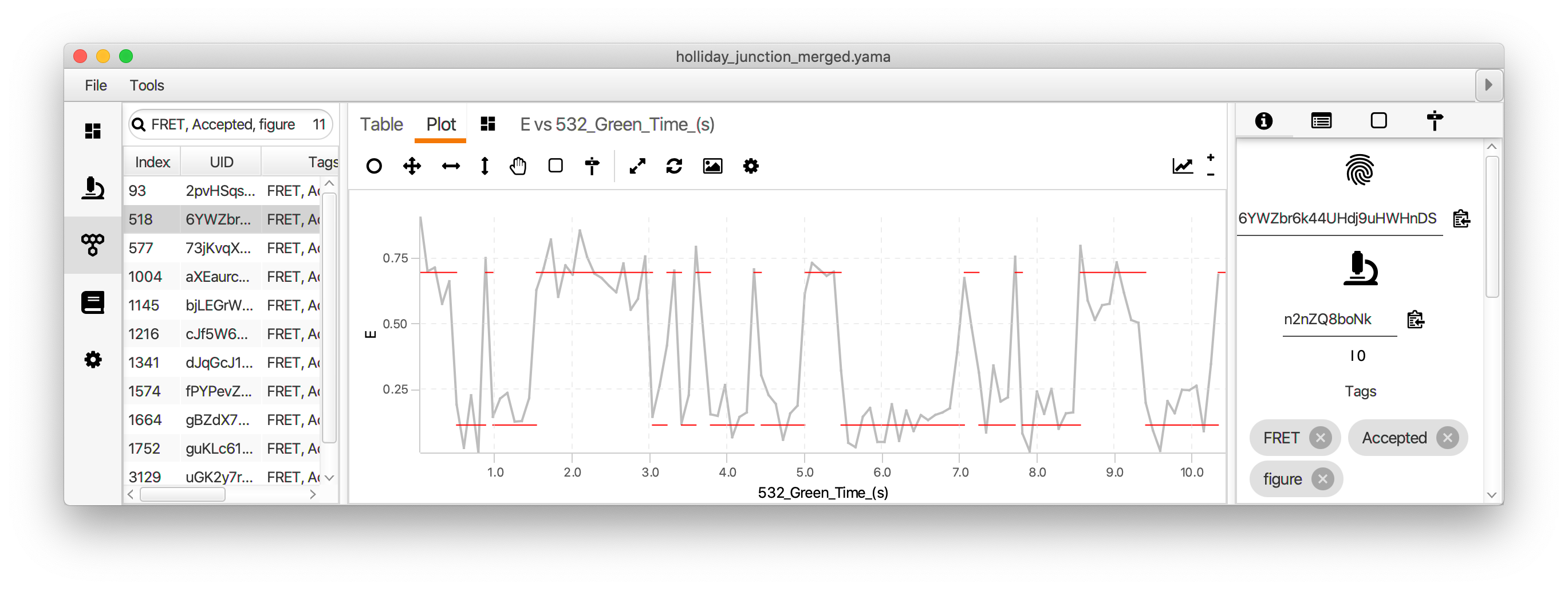
Finally, run the two state fit groovy script to identify the dwells times for each state. This very simple script identifies regions with high and low FRET (E) based using the columns and threshold value provided in the dialog. This should be the fully corrected E values and the time in seconds.

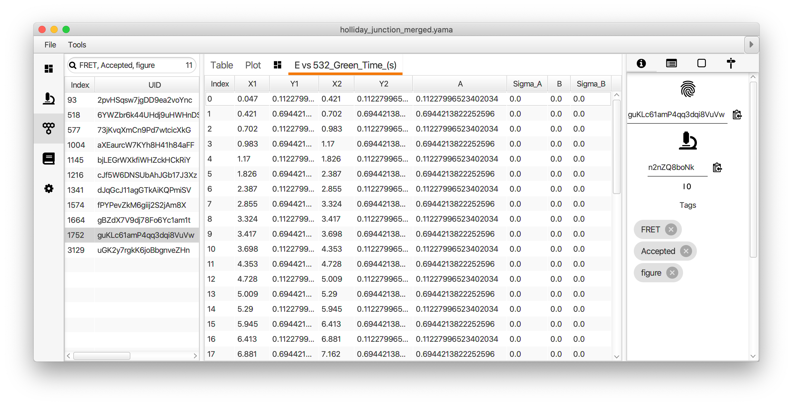
The dwell time information is added to each molecule record as a segments table that shows up in a new tab. This table has the starting and ending coordinates for the segments. The script calculates the mean E value for each state and assigns all segments with that value (A column). The slope of the segments is zero in this case (B column). This column is used for kinetic analysis of tracking results.
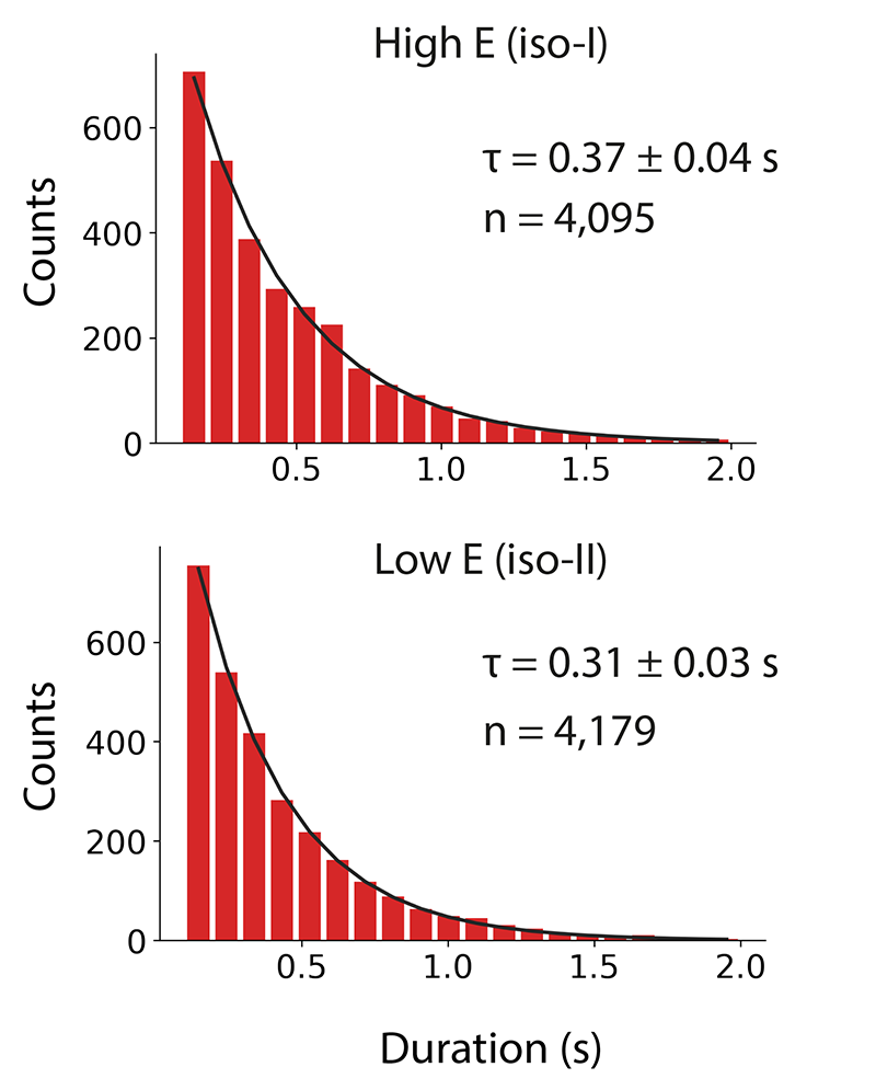
The segments can be viewed in the molecule plot tab by checking the segments box in the plot options panel. The segments will only be displayed if the X and Y columns match those used to generate the segments table. The mean lifetime of each state is determined by fitting the distribution of dwell times for each state with exponential decay function. This is done in Python in the jupyter notebook accompanying this example.
Comments: The two state fit script uses a very simple model that leverages the pre-existing information we have about the system used in this example. The kinetic change point (KCP) command provides a more general option for kinetic analysis that makes no assumptions about the number of states or their E values. The timescale of FRET transitions should be carefully considered. The KCP command, as well as other kinetic analysis tools, provide the best results when the lifetime of FRET states is much longer than the sampling rate. This ensures the FRET states are well resolved over the background noise. The transition rates between FRET states can also be determined using hidden Markov models. Currently, there is no HHM command integrated into Mars. Our suggestion would be to use the python package pomegranate in a jupyter notebook. The results can be added in a segments table and the rate constants as parameters to Mars records. We are working on an example notebook for hidden Markov models. Follow this issue for details. Comment on the issue if you have an urgent need for this.
Exploration in Python
The final Molecule Archive from the steps above is available in the mars-tutorials repository in the files holliday_junction_merged.yama and accompanying holliday_junction_merged.yama.rover.
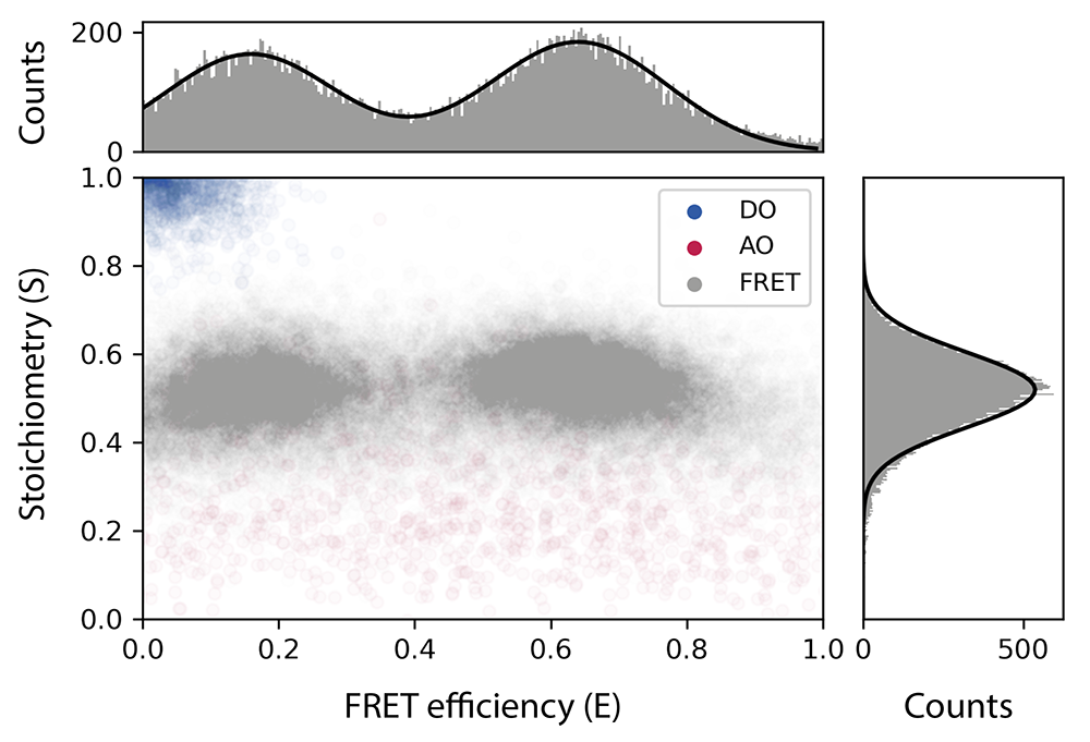
Final distributions are generated using the dynamic FRET example jupyter notebook provided in the mars-tutorials repository. This notebook requires the file path to a local copy of holliday_junction_merged.yama and Fiji as inputs. Please note that running the notebook requires the set-up of a new python environment. Directions to do so can be found in this tutorial. After running all cells several charts are generated showing E and S values for each stage of corrections and the fully correction distributions together with the results of kinetic analysis.
Troubleshooting
This section highlights some of the common errors or problems that may occur during following along with the example as well as possible solutions. Please reference the table below in case you encounter any problems during the analysis. If your question has not been answered in this section, please feel free to reach out to our lab by making a forum post.
| Problem Description | Solution |
|---|---|
| Most parameters (E, S, iEapp, iSapp) display NaN values | This most often happens because some of the metadata tags are missing. Solution: check in the metadata tab if the metadata records are tagged ‘FRET’, ‘AO’, and ‘DO’ respectively. Solution: add the correct tag to the metadata. This problem often arises when the archive has been tagged, but has not been saved, before merging using the Merge Archives command. |
| No peaks were found by the Peak Finder command | This might be the case when the Peak Finder settings (especially threshold settings) are not correct. Solution: verify that the correct Peak Finder settings were entered in the dialog and run the analysis again. |
| The ROI manager is empty after running the Transform ROIs command | This behavior can be caused by two issues: (1) there were no peaks placed in the ROI Manager by the Peak Finder or (2) the ROI Manager was not closed or reset before doing running the transform ROIs command on a second dataset. Solution: (1) check if the Peak Finder settings are entered correctly and use the ‘preview’ option to verify that the command finds the peaks. Check if the ‘Add to ROI Manager’ option is selected in the tab. (2) close the ROI Manager and run the analysis again, starting from the Peak Finder command. |
| The archive or script editor freezes during analysis | We have observed this during develop on rare occasions, especially when the same Fiji session has been active on your computer for a long time. Solution: close Fiji and retry the analysis after a software restart. Saving several copies of the archive during processing is best practive. |
| No I vs. T plots are observed after entering the x and y settings in the plotting menu | Solution: refresh the plot by pressing the refresh button at the bottom right corner of the plot settings menu |
| No output is generated after running a Mars tool | Either the input settings were selected in such a way that no output is expected, or the tool encountered an error. Solution: (1) verify the settings of the tool. (2) Check for red printed errors in the Fiji Console window (Window>Console). Either resolve the error by selecting different settings in the Mars tool dialog window or run the tool again. |
| No changes are made to the Archive after running one of the scripts | It might be that the script encountered an error and did not run till completion. Solution: open the ‘Console’ window (Window>Console) in Fiji and see if any red errors are raised. If so, resolve the error and run the script again. |
References
(1) Hyeon C, Lee J, Yoon J, Hohng S, Thirumalai D. Hidden complexity in the isomerization dynamics of Holliday junctions. Nat Chem. 2012 Nov;4(11):907-14. https://doi.org/10.1038/nchem.1463.